Investigation of the Intricate Universe of Fractals

Fractals Unleashed

Preface

The Mandelbrot set, one of the most iconic objects in modern mathematics, lies at the intersection of fractal geometry, complex dynamics, and topology. Its intricate structure has fascinated mathematicians, physicists, and computer scientists alike, giving rise to various conjectures that seek to explain its deep properties. One such conjecture is the Mandelbrot Locally Connected Conjecture, a longstanding question that posits the local connectedness of the Mandelbrot set at every point. The resolution of this conjecture would enhance our understanding of the set’s boundary, which exhibits extraordinary complexity and serves as the interface between stability and chaos in the dynamics of quadratic polynomials. The Mandelbrot set is not merely a geometric marvel; it plays a pivotal role in the field of complex dynamics, where the behavior of polynomials over complex numbers is studied. In particular, the local connectedness conjecture has profound implications for how the dynamics of these polynomials change as parameters are varied. If proven true, this conjecture would ensure that the boundaries of the Mandelbrot set can be described as connected at every point, facilitating a clearer geometric and topological understanding of the set. Over the years, significant progress has been made in understanding the local properties of the Mandelbrot set. While the conjecture remains unresolved in its most general form, it has been shown to hold in specific regions, especially within hyperbolic components. Techniques from complex analysis, topology, and Teichmüller theory have been central to these advances. Moreover, computational tools and visualizations have allowed researchers to probe the Mandelbrot set’s boundary at unprecedented levels of precision, offering experimental evidence that lends credence to the conjecture.

This preface introduces the reader to the key concepts surrounding the Mandelbrot Locally Connected Conjecture and provides a brief overview of the research landscape. The study of this conjecture is not only about solving a theoretical puzzle—it opens a window into understanding the dynamic behavior of mathematical systems at their most fundamental level. This ongoing exploration represents the intersection of deep theoretical inquiry and cutting-edge computational techniques, promising to shed new light on one of the most beautiful structures in mathematics. This work aims to guide the reader through the significant developments in this area, offering both mathematical insight and context into the ongoing research on this fascinating and intricate conjecture. Moreover, this work aims to guide the reader through the significant developments in this field, highlighting key results, methodologies, and the evolving landscape of research surrounding this conjecture. By offering both mathematical insights and context, the aim is to provide a comprehensive view of the challenges and breakthroughs that characterize the study of the Mandelbrot Locally Connected Conjecture. Through this journey, we hope to illuminate the intricacies of this fascinating and intricate conjecture, inspiring further exploration and curiosity within the realm of complex dynamics.

Introduction

The development of complex dynamics and fractals has evolved from the pioneering work in the early 20th century to its rich modern-day understanding. Complex dynamics began with the studies of Henri Poincaré, who explored the behavior of dynamical systems, laying the foundation for chaos theory. In the 1910s, Pierre Fatou and Gaston Julia investigated the iteration of functions in the complex plane, introducing key concepts such as the Julia set and Fatou set, which describe regions of stability and chaos in dynamical systems. This early work largely went unnoticed until Benoit Mandelbrot popularized fractals in the 1970s. Mandelbrot’s fractal geometry, exemplified by the Mandelbrot set, revealed the self-similar and infinitely complex structures emerging from simple iterative processes.

Pierre Fatou and Gaston Julia two French mathematicians who independently laid the foundation of complex dynamics in the early 20th century, specifically focusing on the iteration of complex functions. They investigated the behavior of complex functions when iterated repeatedly, i.e., applying the same function over and over to a complex number. This led to the development of Julia sets and Fatou sets, which describe the stability and chaotic behavior of points under such iterations.

Understanding By Studying Books & Research Papers

I am currently studying two foundational texts in the field of complex dynamics: “Complex Dynamics” by Lennart Carleson and Theodore Gamelin and “Dynamics in One Complex Variable” by John Milnor. I am gradually gaining a deeper understanding of key concepts in the field of complex dynamics. Though the material is quite challenging, it has offered me valuable insights into the behavior of iterated functions, the formation of Julia sets, and the structure of the Mandelbrot set. My comprehension is evolving, particularly in understanding the intricate relationships between stable and unstable points, and how chaotic behavior emerges in dynamical systems. Furthermore, I am beginning to appreciate the subtle distinctions between holomorphic functions in one complex variable and their dynamical properties. These texts have provided a framework that is helping me grasp the convergence properties and self-similar structures that are fundamental to fractal geometry. The challenge of mastering these ideas is refining my approach to more advanced topics in dynamical systems and fractal analysis, equipping me with the necessary tools to continue exploring this fascinating area of mathematics.

Fatou Sets represent regions in the complex plane where the behavior of the function is stable and predictable. Points in the Fatou set under repeated iterations of the function will exhibit regular or convergent behavior. let’s consider iterating a complex function $f(z)$, where $z$ is a complex number. A simple example of such a function is $f(z)=z^2+c$, where $c$ is a complex constant. The Fatou set $F(f)$ consists of points in the complex plane where the iterations of $f(z)$ are stable, meaning the sequence of iterations remains bounded and does not exhibit chaotic behavior.

Julia Sets represent the boundary of the Fatou set and exhibit chaotic and fractal structures. For a given complex number $c$, the Julia set $J(f)$ of the function $f(z)=z^2+c$ is the set of points $z$ in the complex plane where the function behaves chaotically under iteration. Formally, it’s the boundary between points that tend to infinity and points that remain bounded under infinite iterations.

Let’s take the function $f(z)=z^2+c$, Start with an initial point $z_0$ in the complex plane. Then if we apply $f$ repeatedly: $z_1=f(z_0)=z_0^2+c$, then $z_2=f(z_1)=z_1^2+c$ , and so on. If the points in the complex plane where the sequence $z_n=f^n(z)$ remains bounded i.e., does not tend to infinity the point, $z_0$​ belongs to the Fatou set. If it tends toward infinity or behaves chaotically, $z_0$​ belongs to the Julia set. For $f(z)=z^2-1$, the Julia set will look like a fractal, where points on the set exhibit chaotic behavior under iteration, while points not in the Julia set (the Fatou set) will eventually settle into regular, predictable behavior.

The study of complex dynamics lead us another critical tool in their work is understanding fixed points—points $z$ where $f(z)=z$. Around these fixed points, the behavior of the function can be analyzed using derivatives to determine stability:

• A fixed point $z_0$​ is attracting if $|f^{\prime }(z_0)|<1$ , meaning nearby points will converge to $z_0$​ under iteration.

• It is repelling if $|f^{\prime }(z_0)|>1$ , where nearby points will move away, leading to chaotic behavior typical of the Julia set.

One of the key properties of fractals like Julia sets is their fractal dimension. The fractal dimension $D$ can be thought of as a measure of how the detail in the fractal changes with the scale at which it is viewed. For a self-similar fractal, the dimension is defined mathematically as:

$$D=\frac{\log (N)}{\log (r)}$$​

where $N$ is the number of self-similar pieces the fractal is broken into at a given scale, and $r$ is the scaling factor.

Julia sets often have a non-integer Hausdorff dimension, reflecting their complex, non-Euclidean nature. For example, a Julia set might have a dimension like 1.6, indicating it is more complex than a 1-dimensional line but not fully 2-dimensional.

The iterative nature of Julia sets, where a function $f(z)$ is repeatedly applied to generate complex patterns, can be modeled using Iterated Function Systems (IFS). The structure of fractals emerges from the repeated application of transformations (like scaling, rotating, or translating) to an initial set of points. In the case of Julia sets, the transformation is defined by a complex function, and the resulting fractal emerges as the boundary of points that exhibit chaotic behavior under iteration.

My Investigation

Starting From The Root

Consider, for instance, the simple function $f(z)=z+1.$ In this context, we start with an initial value of $z$and evaluate the function. The result is then used as the new input parameter, and the function is evaluated again. This iterative process can be formally described as follows:

1. Start with an initial value $z_0$​.

2. Compute $z_1=f(z_0)=z_0+1.$

3. Use $z_1$ as the new input to compute $z_2=f(z_1)=z_1+1$, and so forth.

Mathematically, this generates a sequence $\{z_n\}$ where $z_{n+1}=f(z_n)=z_n+1.$ This sequence clearly grows without bound, illustrating a simple yet profound example of iterative processes in dynamical systems. Such iterations lay the groundwork for understanding more complex functions and their behaviors, which ultimately lead to the rich, intricate patterns observed in fractals.

Finally we’ll see that,

$$f(0)=0+1=1$$

$$f(1)=1+1=2$$

$$f(2)=2+1=3$$

$$\text{and so on}\dots$$

The pattern here is straightforward: we evaluate the function, use the result as the new input, and re-evaluate the function. In this simple case, observing the pattern is easy, as the value increases by one with each iteration. While this example is quite basic, Mandelbrot extended this concept significantly further.

Mandelbrot studied the function $f(z)=z^2+c$. To illustrate this with a simple example, let’s choose $c=1$. Therefore,

$$f(0)=1$$

$$f(1)=2$$

$$f(2)=5$$

$$f(5)=26$$

It becomes apparent that the values will rapidly spiral out of control this time and diverge to infinity. Now let’s try plugging in $-2$. Therefore,

$$f(0)=-2$$

$$f(-2)=2$$

$$f(2)=2$$

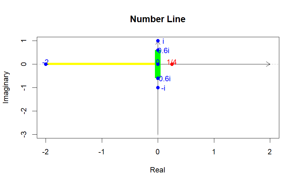
This process will continually yield the value $2$. By repeatedly evaluating $f(2)$ and obtaining $2$, this iteration continues indefinitely. Consequently, this indicates that $-2$ lies on the boundary of the Mandelbrot set. To visualize this concept, let’s draw a number line.

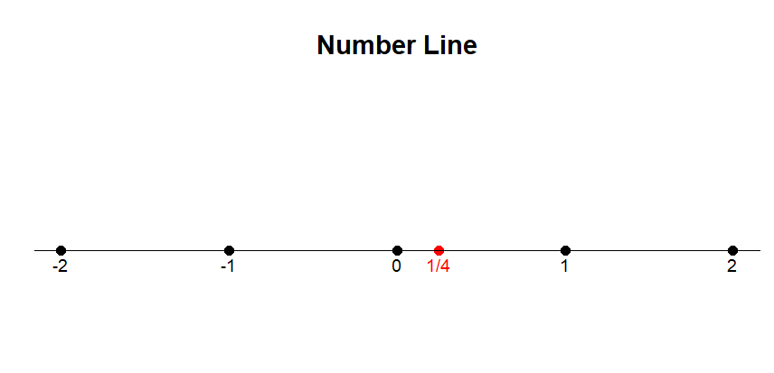
Here, $-2$ represents the largest magnitude that remains bounded and does not diverge to infinity when iterated from $0.$

Let’s try plugging, $c=-2.1$. Therefore,

$$f(0)=0^2-2.1=-2.1$$

$$f(-2.1)=(-2.1{)}^2-2.1=2.41$$

$$f(2.41)=(2.41{)}^2-2.1=3.81$$

$$f(3.81)=(3.81{)}^2-2.1=12.5$$

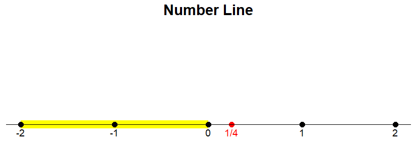
Consider the parameter $c=-2.1.$ Through successive iterations of the function $f(z)=z^2+c$, we embark on a journey: $-2.1,2.41,3.81,12.5$, and so forth, each value exponentially greater than the last. This vividly illustrates that the Mandelbrot set’s boundary is encapsulated by $-2$, beyond which values spiral into infinity. Now, let’s shift our focus to the positive boundary. Surprisingly, it resides at $c=\frac{1}{4}$, a less intuitive revelation. When we substitute $\frac{1}{4}$ for $c$, the sequence inches closer and closer to $\frac{1}{2}$, but never quite reaches it. Any departure beyond $\frac{1}{4}$ propels the sequence into an unbounded trajectory towards infinity. We may visually represent this by shading the region between these two values on a number line, symbolizing the real numbers encompassed by the Mandelbrot set. The interval stretches from $-2$ to $\frac{1}{4}$​, delineating the scope of this fractal phenomenon. At this juncture, some individuals might conclude their exploration. However, what follows promises a journey into deeper complexity.

Analysing Julia Set

In the early ${20}^{\text{th}}$ century mathematicians, Pierre Fatou and Gaston Julia set the stage for the discovery of the Mandelbrot set with their exploration of Dynamical Systems. To investigate these dynamical systems, mathematicians study intricate shapes which is known as Julia Sets. Julia Sets are produced by iterating a function of complex numbers.

A complex number is defined as the sum of two components, a real part and an imaginary part. Each complex number can be visualized as a point of a 2D plane. The real part is a number found on the number line. The imaginary part is a multiple of the $\sqrt{-1}$, which the mathematicians write as $i$. Despite the name, imaginary numbers play a vital role in solving real-world problems. To construct Julia Set, start with a simple quadratic equation $f(z)=z^2+c$

For example, choose a value for c = -1. Then consider what happens when you iterate this equation for every possible starting value. You repeatedly apply the function to the sequence of numbers that you’re generating, and you ask whether or not that sequence is going off to infinity or whether it stay bounded. - Laura Demarco (Mathematician, Havard)

For some initial values, your equation speeds off to infinity while iterating like these.These values are not in the Julia set. When you start iterating from other initial values, you might instead get a sequence of outputs that stay bounded.

When something comes back to itself, we often call that recurrent behaviour, & that’s where the complexity arises.

The boundary between points that stay bounded and those that don’t is a Julia set. You can fill it in by including all the bounded values.

Julia sets are certain fractal sets in the complex plane that arise from the dynamics of complex polynomials.

The Filled Julia Set

Consider a polynomial map $f:\mathbb{C}\to \mathbb{C}$, such as $f(z)=z^2-1$. What are the dynamics of such a map?Certainly, many orbits under this map diverge to infinity:

$$p_1=2,p_2=3,p_3=8,p_4=63,p_5=3968,\dots$$

On the other hand, some orbits manage to remain bounded:

$$p_1=0.5,p_2=-0.75,p_3=-0.4375,p_4\approx -0.8086,\dots$$

Definition: Types of Orbits

Let $f:\mathbb{C}\to \mathbb{C}$ be a polynomial map, and let $\{p_1,p_2,p_3,\dots \}$ be an orbit under $f$.

1. We say that the orbit is bounded if all the points are contained in some disk of finite radius centered at the origin. That is, the orbit is bounded if there exists a constant ( $R>0$ ) so that ( $|p_n|\le R$ ) for all $n\in \mathbb{N}$ .

2. We say that the orbit escapes to infinity if ($|p_n|\to \mathrm{\infty }$) as ($n\to \mathrm{\infty }$).

This leads to the question: for what initial points ( $p_1$ ) will the orbit under ( $f$ ) remain bounded, and for what initial points will the orbit escape to infinity?

Definition: Filled Julia Set / Basin of Infinity

Let $f:\mathbb{C}\to \mathbb{C}$ be a polynomial map.

1. The filled Julia set for $f$ is the set:

$$p_1\in \mathbb{C}|\text{the orbit of }{p}_1\text{ is bounded}.$$

2. The basin of infinity for ( $f$ ) is the set:

   $$p_1\in \mathbb{C}|\text{the orbit of }{p}_1\text{ escapes to infinity}.$$

Example 1: Repeated Squaring

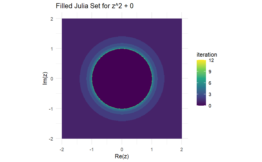
Let $f:\mathbb{C}\to \mathbb{C}$ be the map $f(z)=z^2.$ As we have seen, $f$ squares the radius and doubles the angle of any complex number:

$$f(r{e}^{i\theta })=r^2{e}^{i(2\theta )}.$$

Given an initial point $p_1$, the orbit $\{p_1,p_2,p_3,\dots \}$ has the following behavior, depending on the relationship of $p_1$ to the unit circle:

1. If $|p_1|<1$, then the orbit converges to $0$, which is an attracting fixed point for $f$.

2. If $|p_1|=1$, then the entire orbit lies on the unit circle.

3. If $|p_1|>1$, then the orbit escapes to infinity.

The orbits remain bounded in the first two cases, so the filled Julia set for $f$ is the closed unit disk $\{z\in \mathbb{C}:|z|\le 1\},$ shown in Figure a. The basin of infinity is the complement of this disk.

(a) Filled Julia set for $z^2$

(b) Filled Julia set for $z^2-\frac{4}{9}$

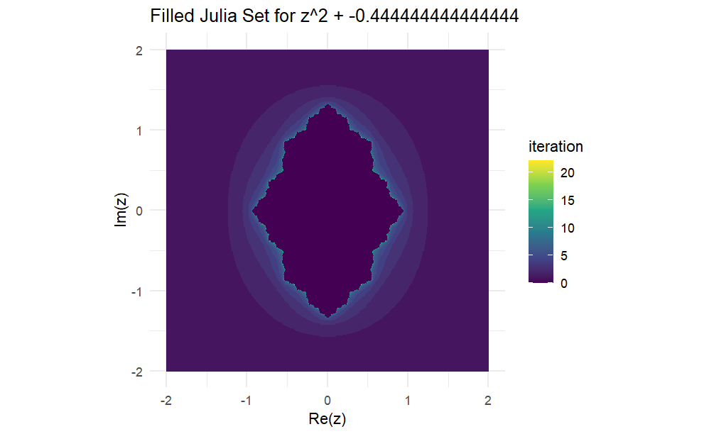
Example 2: The Function ( $z^2-\frac{4}{9}$ )

Let $f:\mathbb{C}\to \mathbb{C}$ be the function $f(z)=z^2-\frac{4}{9}.$ Since,

$$f(-\frac{1}{3})=-\frac{1}{3}\text{and}|f^{\prime }(-\frac{1}{3})|=|-\frac{2}{3}|<1,$$

this function has an attracting fixed point at $-\frac{2}{3}$

The filled Julia set for f is shown in Figure(b). The dynamics of $f$ are very similar to the dynamics of the squaring map: the orbit of any point in the interior of the filled Julia set converges to the fixed point, while the orbit of any point outside the filled Julia set escapes to infinity. Points that lie precisely on the boundary of the filled Julia set remain on the boundary as the map is iterated.

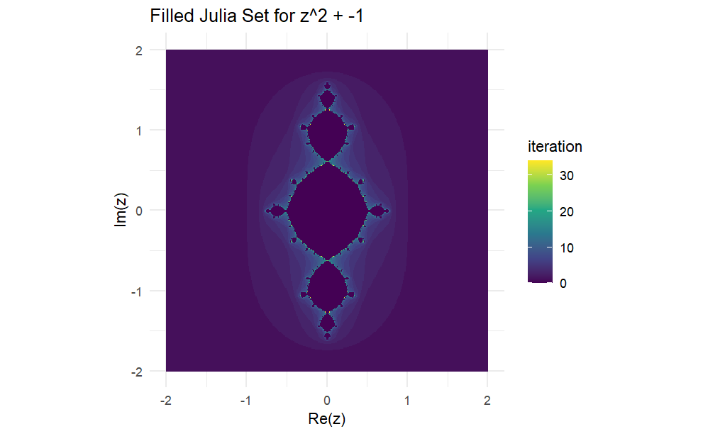
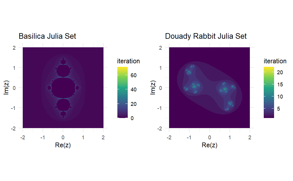
Example 3: The Basilica and the Rabbit

Let $f:\mathbb{C}\to \mathbb{C}$ be the function $f(z)=z^2-1.$ Although this function does not have an attracting fixed point, it is easy to check that:

$$f(0)=-1,f(-1)=0,\text{and}|f^{\prime }(0)f^{\prime }(-1)|=|(0)(-2)|=0<1,$$

$$\text{so}\{-1,0\}\text{is an attracting two-cycle}.$$

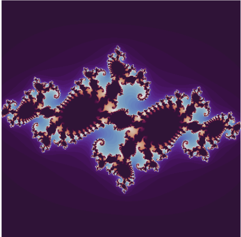
The filled Julia set for this function is shown in figure below. The filled Julia set for this function is known as the Basilica, because of its resemblance to St. Peter’s Basilica. Orbits of points in the interior of the filled Julia set are attracted to the 2-cycle, while orbits of points outside escape to infinity. As with the previous examples, the orbit of any point precisely on the boundary of the filled Julia set remains on the boundary.

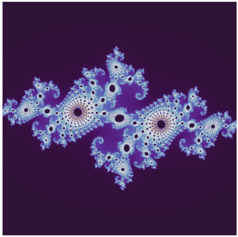
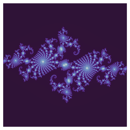
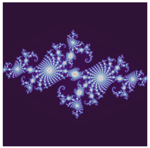
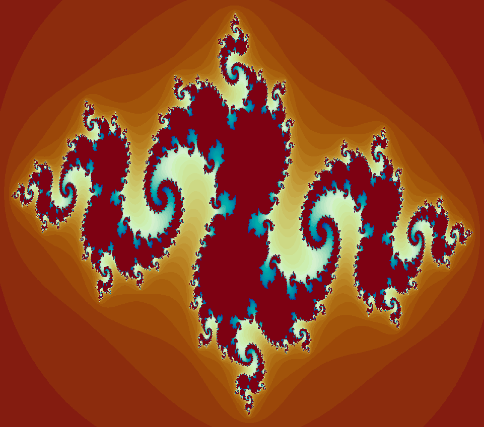
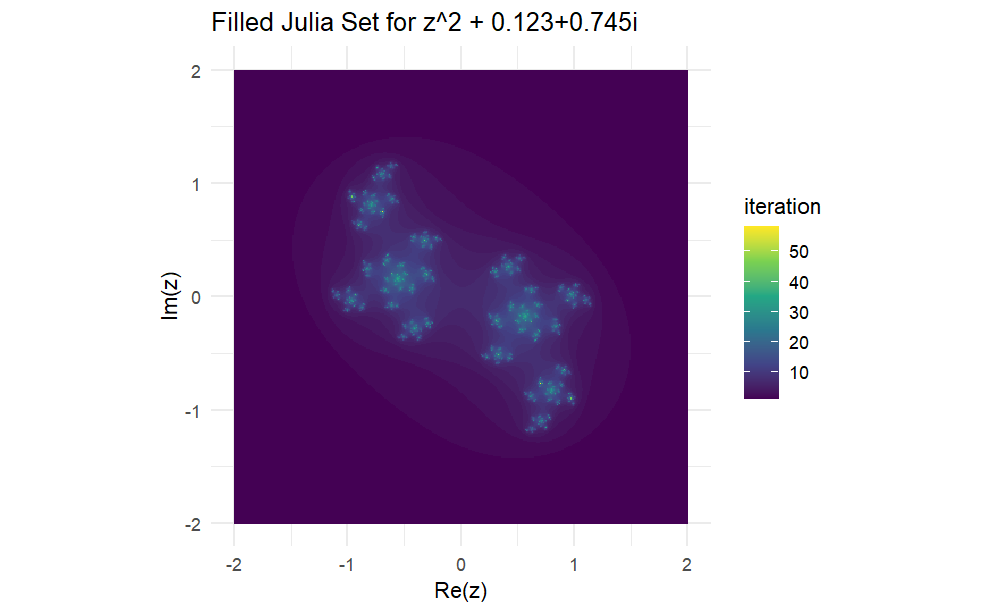
Another function with similar dynamics is the quadratic $f(z)=z^2-0.123+0.754i$ . This polynomial has an attracting 3-cycle, and most orbits either asymptotically approach the 3-cycle or escape to infinity. The filled Julia set for this function is known as the Douady rabbit, named after the French mathematician Adrien Douady.

Properties of the Filled Julia Set

Let $f:\mathbb{C}\to \mathbb{C}$ be a polynomial function. Let $B$ be the basin of infinity for $f$ , and let $J$ be the filled Julia set for $f$. Then:

1. $B$ and $J$ are disjoint, and $B\cup J=\mathbb{C}$.

2. Both $B$ and $J$ are invariant under $f,$ i.e., $f(B)=B$ and $f(J)=J$.

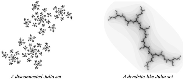
Filled Julia sets can be divided into two categories. Sets are connected so that you can draw a line from one point to another without lifting your pen. Sets where points look like scattered pieces of dust are disconnected.

Elementary Complex Number

Let’s quickly explore the realm of complex numbers. The square root function identifies a number which, when multiplied by itself, yields the number under the radical. For instance, $\sqrt{4}$​ implies that since $2$ times itself is $4$, $\sqrt{4}$ is $2$.

Now, let’s consider the square root of a negative number. For example, what if we have $\sqrt{-4}$? Can you identify a number which, when multiplied by itself, equals $-4$?

The answer is you can’t, because there are no real numbers that satisfy this condition. This is because the square of any real number is always non-negative.

Similar questions arise with $\sqrt{-1}$​. What is the square root of $-1$?

The answer is that there are no real numbers that satisfy this condition. To address this, mathematicians introduced the concept of imaginary numbers. The square root of -1 is defined as $i$, where $i$ is the imaginary unit. Also, now we can answer about $\sqrt{-4}$ i.e., $\sqrt{-4}=2i\times 2i=(2.2)\times (i.i)=-4$.

Extension of $f(z)=z^2+c$ With Imaginary Number

So, Mandelbrot wanted to Inlcude imaginary numbers as well in his analysis of his function.

$$f(z)=z^2+c$$

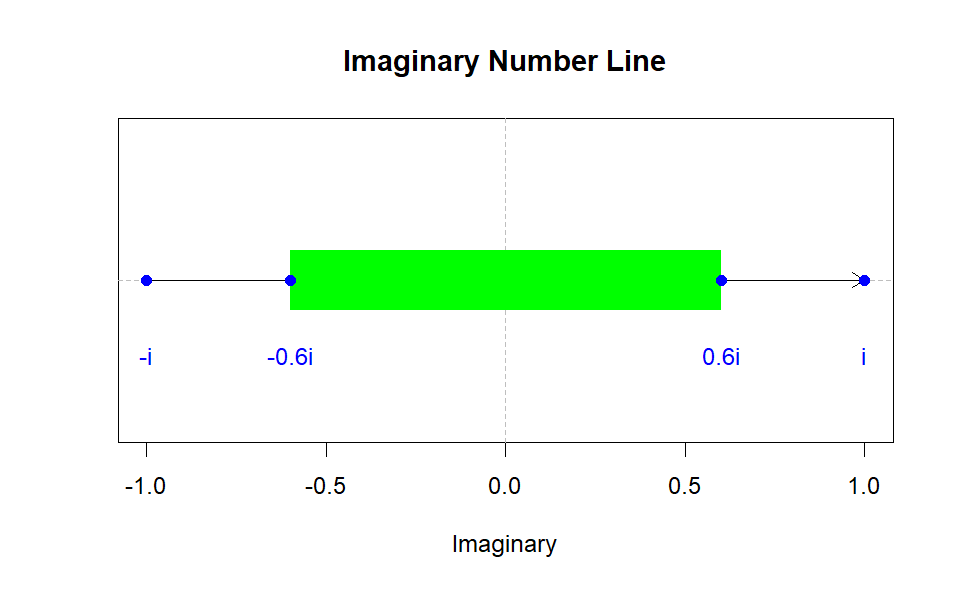
Let’s try plug in $i$ for $c$ i.e., $c=i$.

$$f(0)=i$$

$$f(i)=(i{)}^2+1=-1+i$$

$$f(-1+i)=(-1+i{)}^2+i=-i$$

Continuing the iterations by hand becomes increasingly complex, so we will pause here. It’s important to note that $i$ is not included in the Mandelbrot set, as this function diverges to infinity. To visualize this, we can set up an imaginary number line. The bounds for this function are approximately $-0.6i$ & $0.6i$

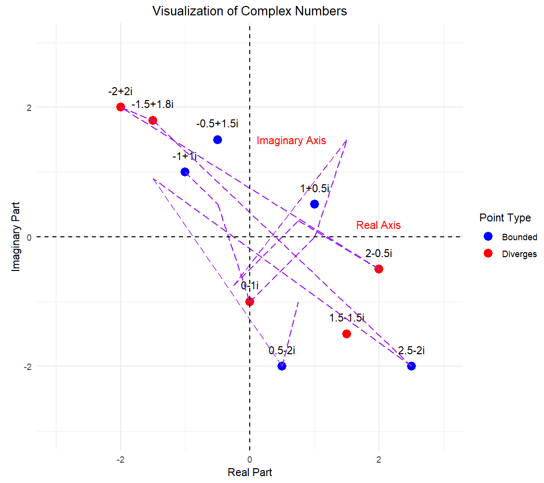
Many mathematicians might have stopped at this point, having defined the set for all real numbers and all imaginary numbers. However, there remains one more set of numbers to explore: complex numbers. Complex numbers consist of both a real and an imaginary component. This extension allows us to include complex numbers in our number system. A complex number can be expressed in the form $a+bi$, where $a$ and $b$ are real numbers. This could be something as simple as $1+i$ or as complex as $6+9i$. If we let 𝑐c be any complex number, it can represent any combination of real and imaginary components.

Roughly $-0.2+1.12i$ is included in the Mandelbrot set

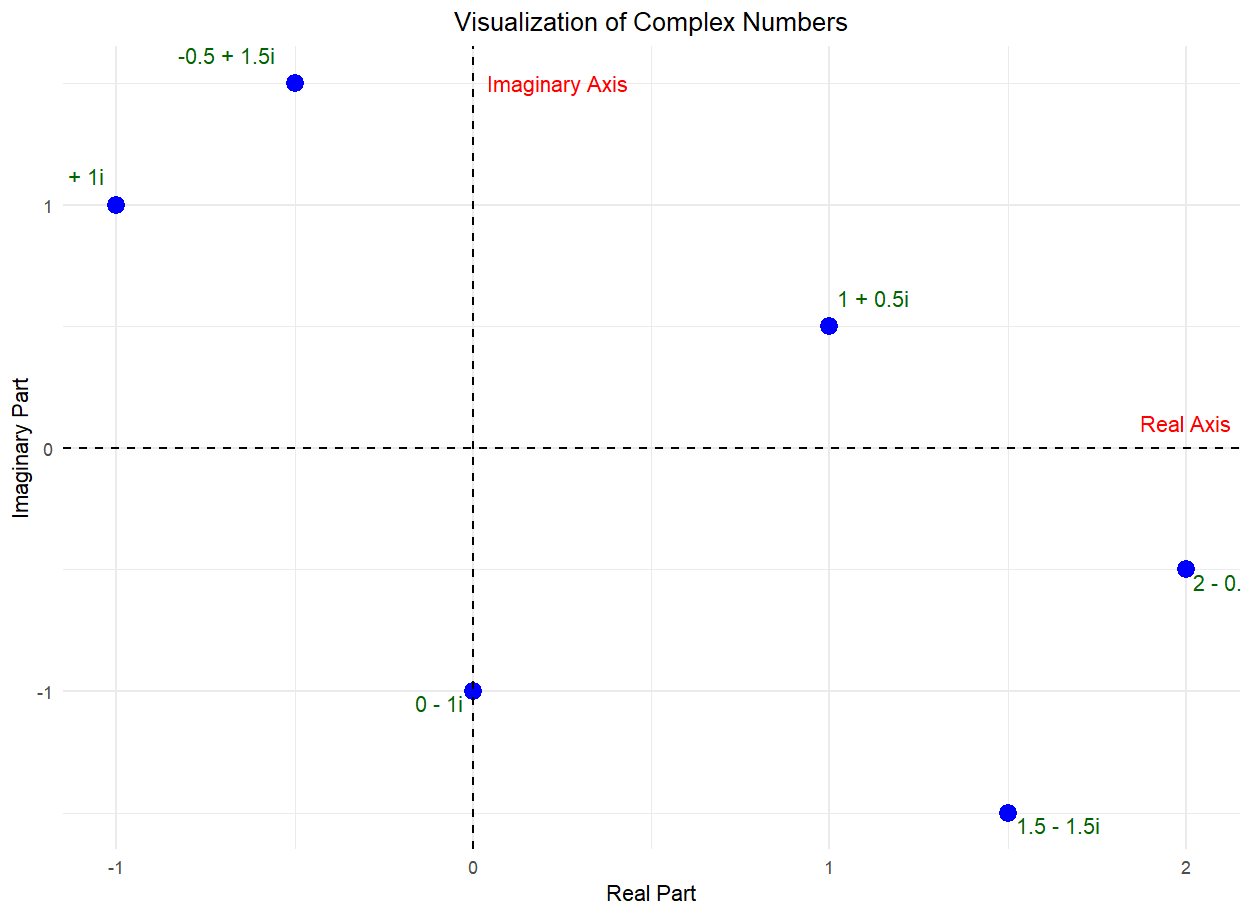
But where do we place this on the number line? We can’t simply put it above $-0.2$ because we have $0.2+1.12i$, where the real part is $-0.2.$ If only there were some way to simultaneously represent both real and imaginary components. We need something like this:

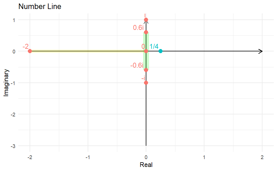
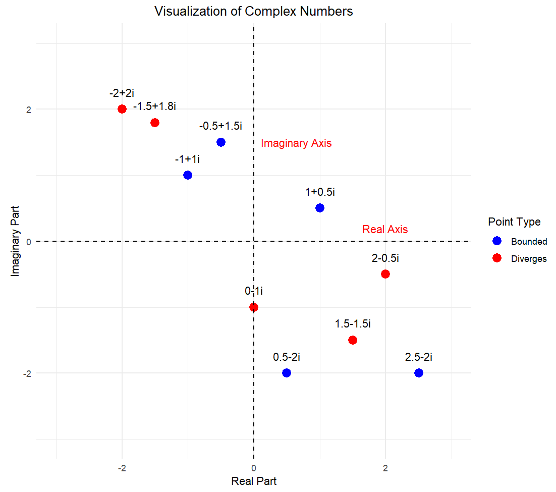
In this complex plane, we can plot complex numbers in the form $a+bi$. The horizontal axis (real axis) represents the real part $a$, and the vertical axis (imaginary axis) represents the imaginary part $bi$. In this complex plane, each point $(a,b)$ corresponds to the complex number $a+bi$. This way, both the real and imaginary parts of the number can be viewed together.

The Discovery of The Mandelbrot Set

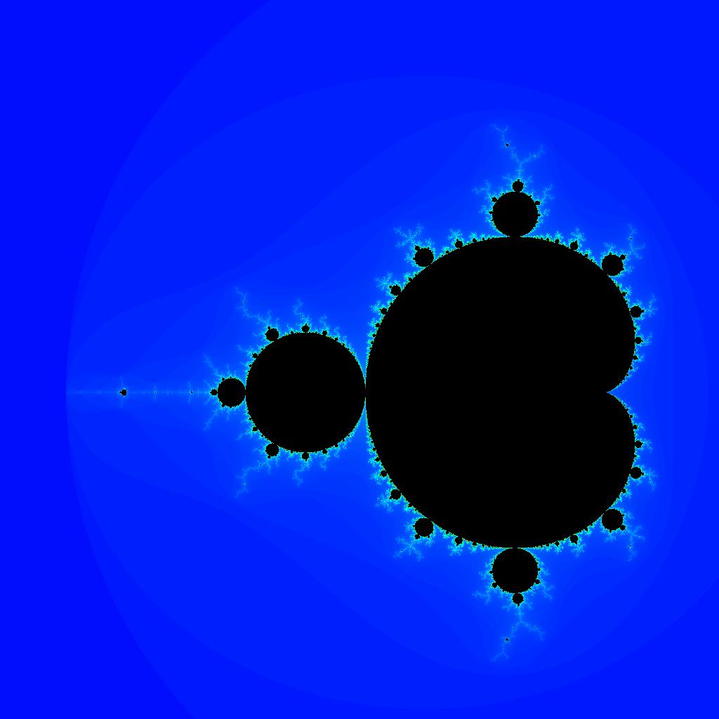
The first rough plot of the Mandelbrot set appeared in a 1978 paper by the mathematicians Robert Brooks and J. Peter Matelski. Soon after Benoit Mandelbrot, a researcher at IBM, who had access to more computing power, also discovered the set. This led to further explorations. These early computer graphics were crude, but the patterns revealed the presence of something far more complex.

Even with fuzzy, poorly made pictures in the eighties, they were able to glean a lot of interesting insight into what was going on.

Mandelbrot went on to popularize his now-eponymous set to the world and became known as the father of fractals. Today mathematicians can use computers to explore the Mandelbrot set in far greater detail.

As soon as you have the images just opens up this whole world.

The Mandelbrot set is drawn in the complex plane. It is constructed by iterating the same quadratic equations used to produce Julia sets. But here things are flipped around. Instead of iterating all values of $z$ for a fixed value of $c$, we fix the starting value of the iteration at $0$ and vary $c$. Value of $c$ where iteration of $z^2+c$ stays bounded inside the Mandelbrot set. while those that go to infinity are not.

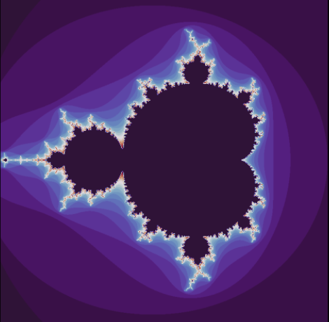
The Mandelbrot set is a perfect example of how a simple rule can produce incredible complexity. At it’s core the set is generated by iterating a quadratic equation, $f(z)=z^2+c$, a simple formula whose highest exponent is $2$. To iterate a quadratic equation, choose a value for the variable, plug it into the function, then take the output and feed it back in again and again. The study of how recursive functions like these changes over time is central to a field of math called ‘Complex Dynamical Systems’.

Studying of Mandelbrot Set

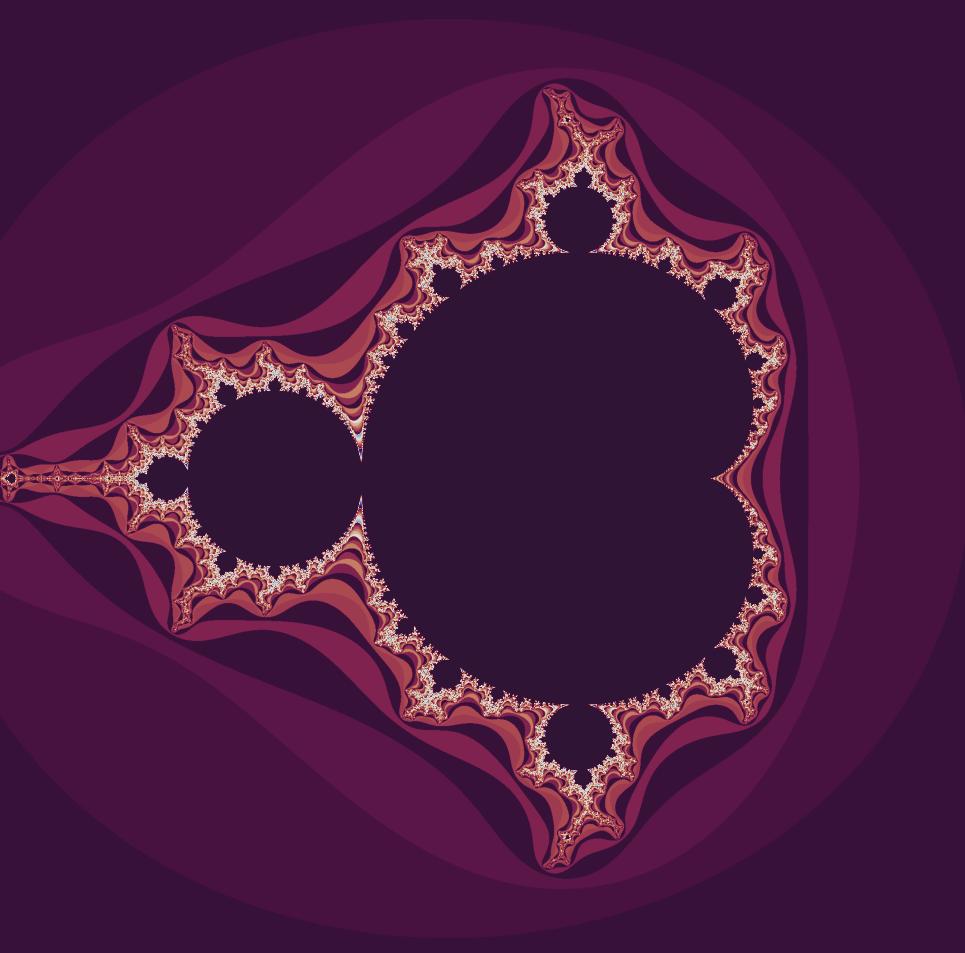
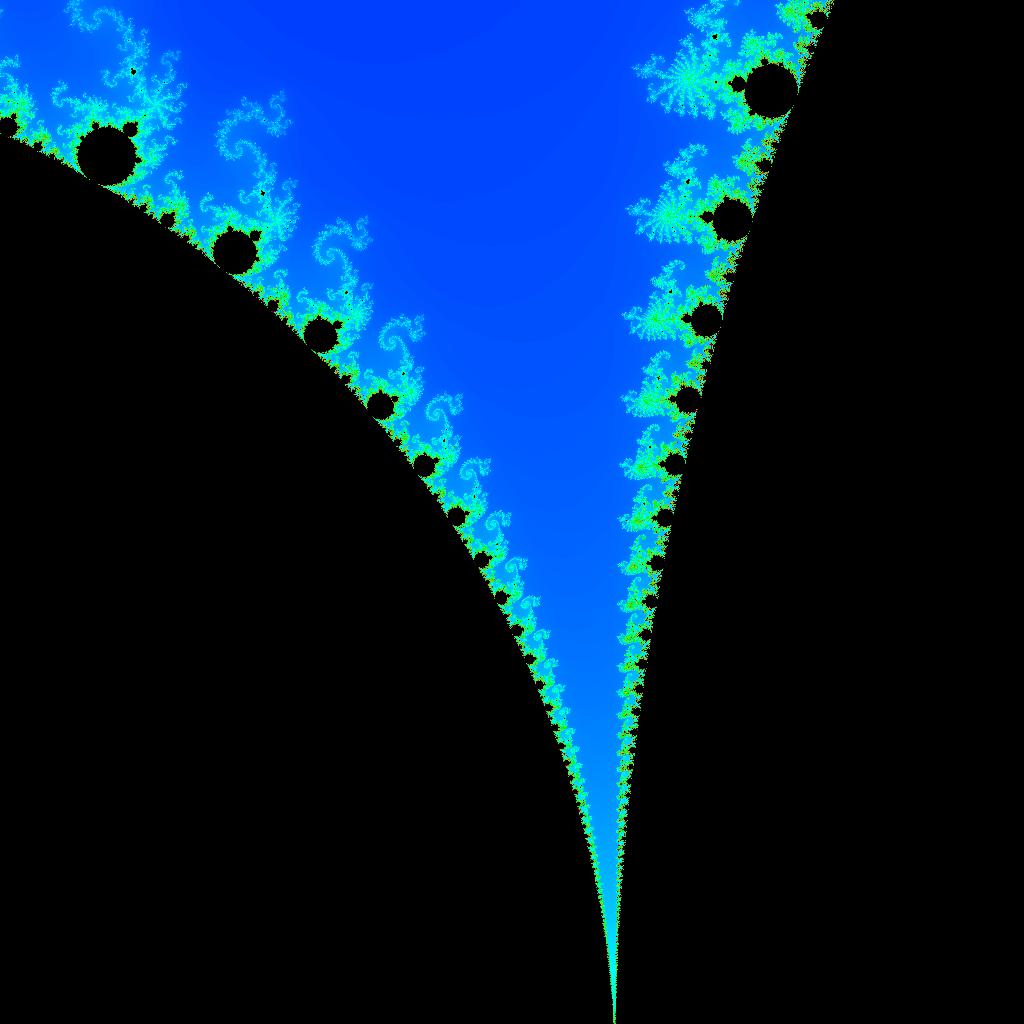
This subject emerged to comprehend the tangible world. What mathematical principles underlie the physical realities we observe? One of the earliest and most crucial examples is the solar system. We delve into dynamical systems, where a set of rules governs the evolution of a space over time, determining the movements and transformations within it. The Mandelbrot set has many intriguing features, but the biggest mysteries lie in its complex fractal boundary. Zooming into different boundary regions reveals some astounding features. A valley of seahorses, parades of elephants and a miniature version of the set itself.

So, we can sort of keep finding nests, a sequence of smaller and smaller Mandelbrot sets. all one inside of the next.

Here at the boundary, mathematicians are probing for answers.

Mandelbrot Locally Connected Conjecture(MLC)

The Mandelbrot Locally Connected Conjecture posits that the Mandelbrot set is locally connected at every point. This conjecture is significant in complex dynamics and has implications for the understanding of the intricate structures of the Mandelbrot set and its Julia sets. This question is central to a 40-year-old problem called the Mandelbrot Locally Connected Conjecture(MLC). If the set is locally connected, that means that no matter what point you choose to examine or how far you zoom in, the are will always look like one nice connected section.

For example, if we closely examine a circle, we can see that it’s locally connected a every point, but take a fine-toothed comb and zoom in while the comb is one connected shape, at close range, it can look disconnected. If mathematicians can prove that MLC is true then a complete understanding of the Mandelbrot set would be within reach.

Mathematical Overview

The Mandelbrot set $M$ is defined in the complex plane as follows:

$$M=\{c\in \mathbb{C}|\text{the sequence defined by }{z}_{n+1}=z_n^2+c\text{ with }{z}_0=0\text{ is bounded}\}$$

• Connectedness: The set is connected and exhibits intricate fractal structures.

• Boundary: The boundary of the Mandelbrot set is infinitely complex and is where most of the interesting dynamics occur.

Locally Connected Conjecture

The conjecture states that every point in the Mandelbrot set is locally connected. In other words, for every point $c$ in $M$ and every neighborhood around $c$, there exists a smaller neighborhood that remains within MMM.

Formal Definition:

• A space is locally connected if for every point in the space and every neighborhood of that point, there exists a connected neighborhood contained within that neighborhood.

Implications of the Conjecture

1. Structure of Julia Sets: If the Mandelbrot set is locally connected, it implies that the Julia sets for parameters $c$ near points in $M$ are also locally connected, leading to clearer geometric interpretations of their structures.

2. Understanding Dynamics: Local connectedness provides insights into how the dynamics change as we move through the parameter space of $c$.

Research Developments

Ongoing research on the Mandelbrot locally connected conjecture involves various approaches, including:

1. Complex Analysis and Topology: Techniques from these fields are utilized to investigate the properties of the Mandelbrot set and its local behavior.

2. Parameter Space Analysis: Researchers study the behavior of the Mandelbrot set in relation to its parameter space and how small changes in ccc affect the connectivity of the set.

3. Computational Approaches: Numerical experiments and visualizations provide insights and help test the conjecture. Researchers often use high-resolution computer graphics to analyze the boundaries of the Mandelbrot set.

4. New Theorems and Techniques: The development of new mathematical tools, such as teichmüller theory, has been instrumental in advancing the understanding of the Mandelbrot set’s structure.

Key Results

Some key results related to the Mandelbrot locally connected conjecture include:

• The conjecture has been shown to hold true for many specific regions of the Mandelbrot set, particularly in the so-called hyperbolic components.

• Research has demonstrated that if the conjecture holds for all parameters in a connected region, it may extend to the entire set, although this remains a point of contention and investigation.

Project on Iterated Function System

Analyzing Fractal Complexity

The Project was a comprehensive examination of iterated function systems in Mathematical and Computational Sciences. Here, our analysis based upon fractal’s complexity using Iterated Function System(IFS) in that project we investigated Iterated Function Systems (IFS), a mathematical framework within fractal geometry used to generate intricate, self-replicating patterns. The project focuses on how contraction mappings iteratively transform points within a space, leading to the convergence of points into a fractal structure known as the limit set. The study examines the role of probability weights in influencing transformations and explores the visual complexity that emerges from simple mathematical functions. Applications of IFS, particularly in computer graphics and image compression, are also highlighted. The conclusion emphasizes the potential for deeper research by modifying constraints, parameters, and probability vectors to refine aesthetic control and enhance the generation of complex geometric patterns. This investigation bridges mathematical principles and artistic expression, suggesting future interdisciplinary collaborations between mathematicians, artists, and computer scientists to push the creative boundaries of generative algorithms.

Chaos Game For The Barnsley Fern

The chaos game is an engaging and intuitive way to explore the fractal structures generated by IFS transformations. By iteratively applying random transformations to points in a space, you can observe the emergence of intricate and self-replicating patterns. In a research or coding project focused on IFS, incorporating the chaos game serves both educational and practical purposes. Here are some points you might consider emphasizing or exploring further.

The fern is one of the basic examples of self-similar sets, i.e. it is a mathematically generated pattern that can be reproducible at any magnification or reduction. Barnsley’s 1988 book Fractals Everywhere is based on the course that he taught for undergraduate and graduate students in the School of Mathematics, Georgia Institute of Technology, called Fractal Geometry. After publishing the book, a second course was developed, called Fractal Measure Theory. Barnsley’s work has been a source of inspiration to graphic artists attempting to imitate nature with mathematical models. The fern code developed by Barnsley is an example of an iterated function system (IFS) to create a fractal. This follows from the collage theorem. He has used fractals to model a diverse range of phenomena in science and technology, but most specifically plant structures. Barnsley’s fern uses four affine transformations. The formula for one transformation is the following:

$$f(x,y)=\left[\begin{array}{ccc}a& b& \\ c& d\end{array}\right]\left[\begin{array}{c}x\\ y\end{array}\right]+\left[\begin{array}{c}e\\ f\end{array}\right]$$

Barnsley shows the IFS code for his Black Spleenwort fern fractal as a matrix of values shown in a table. In the table, the columns “a” through “f” are the coefficients of the equation and “p” represents the probability factor.

We have written the assumption that the functions are defined over a two dimensional space with $x$ and $y$ coordinates, but it generalizes naturally to any number of dimensions. When choosing a transformation function in step 3, you can sample uniformly at random, or impose a bias so that some transformation are applied more often than others. To get a sense of how this works, let’s start with a classic example: the Barnsley fern. The Barnsley fern, like many iterated function systems used for the art, is constructed from functions $f(x,y)$ defined in two dimensions. Better yet, they’re all affine transformations. So we write any such function down using good old fashioned linear algebra, and compute everything using matrix multiplication and addition:

$$f(x,y)=\left[\begin{array}{ccc}a& b& \\ c& d\end{array}\right]\left[\begin{array}{c}x\\ y\end{array}\right]+\left[\begin{array}{c}e\\ f\end{array}\right]$$

Four functions build the Barnsley fern, with the coefficients listed below:

function	$a$	$b$	$c$	$d$	$e$	$f$	$p$	interpretation
$f_1(x,y)$	0	0	0	0.16	0	0	0.01	stem
$f_2(x,y)$	0.85	0.04	-0.04	0.85	0	1.60	0.85	ever-smaller leaflets
$f_3(x,y)$	0.20	-0.26	0.23	0.22	0	1.60	0.07	largest left-hand leaflet
$f_4(x,y)$	-0.15	0.28	0.26	0.24	0	0.44	0.07	largest right-hand leaflet

$$f_1(x,y)=\left[\begin{array}{ccc}0.00& 0.00& \\ 0.00& 0.16\end{array}\right]\left[\begin{array}{c}x\\ y\end{array}\right]$$

$$f_2(x,y)=\left[\begin{array}{ccc}0.85& 0.04& \\ -0.04& 0.85\end{array}\right]\left[\begin{array}{c}x\\ y\end{array}\right]+\left[\begin{array}{c}0.00\\ 1.60\end{array}\right]$$

$$f_3(x,y)=\left[\begin{array}{ccc}0.20& -0.26& \\ 0.23& 0.22\end{array}\right]\left[\begin{array}{c}x\\ y\end{array}\right]+\left[\begin{array}{c}0.00\\ 1.60\end{array}\right]$$

$$f_4(x,y)=\left[\begin{array}{ccc}-0.15& 0.28& \\ 0.26& 0.24\end{array}\right]\left[\begin{array}{c}x\\ y\end{array}\right]+\left[\begin{array}{c}0.00\\ 0.44\end{array}\right]$$

The first point drawn is at the origin $(x_0=0,y_0=0)$ and then the new points are iteratively computed by randomly applying one of the following four coordinate transformations:

ƒ₁

$x_{n+1}$ = 0

$y_{n+1}$ = 0.16 y_n

This coordinate transformation is chosen 1% of the time and just maps any point to a point in the first line segment at the base of the stem. In the iterative generation, it acts as a reset to the base of the stem. Crucially it does not reset exactly to $(0,0)$ which allows it to fill in the base stem which is translated and serves as a kind of “kernel” from which all other sections of the fern are generated via transformations ${ƒ}_2,{ƒ}_3,{ƒ}_4.$

ƒ₂

$x_{n+1}$ = 0.85 x_n + 0.04 y_n

$y_{n+1}$ = −0.04 x_n + 0.85 y_n + 1.6

This transformation encodes the self-similarity relationship of the entire fern with the sub-structure which consists of the fern with the removal of the section which includes the bottom two leaves. In the matrix representation, it can be seen to be a slight clockwise rotation, scaled to be slightly smaller and translated in the positive y direction. In the iterative generation, this transformation is applied with probability 85% and is intuitively responsible for the generation of the main stem, and the successive vertical generation of the leaves on either side of the stem from their “original” leaves at the base.

ƒ₃

$x_{n+1}$ = 0.2 x_n − 0.26 y_n

$y_{n+1}$ = 0.23 x_n + 0.22 y_n + 1.6

This transformation encodes the self-similarity of the entire fern with the bottom left leaf. In the matrix representation, it is seen to be a near-90° counter-clockwise rotation, scaled down to approximately 30% size with a translation in the positive y direction. In the iterative generation, it is applied with probability 7% and is intuitively responsible for the generation of the lower-left leaf.

ƒ₄

$x_{n+1}$ = −0.15 x_n + 0.28 y_n

$y_{n+1}$ = 0.26 x_n + 0.24 y_n + 0.44

Similarly, this transformation encodes the self-similarity of the entire fern with the bottom right leaf. From its determinant it is easily seen to include a reflection and can be seen as a similar transformation as ƒ₃ albeit with a reflection about the y-axis. In the iterative-generation, it is applied with probability 7% and is responsible for the generation of the bottom right leaf.

Furthur Research Goals

• The Mandelbrot locally connected conjecture is a profound and active area of research in complex dynamics. While the conjecture remains unproven for the entire Mandelbrot set, significant progress has been made in understanding the local properties of the set and its implications for related areas in mathematics. My current research interests include exploring the Mandelbrot Locally Connected Conjecture (MLC), a central problem in fractal geometry.

• I am also intrigued by holomorphic dynamics in several variables, particularly in the study of higher-dimensional Julia and Fatou sets, where the geometry becomes far more complex and less understood compared to the 1D case. The classification and structure of Fatou components in higher dimensions remain topics of ongoing research. Additionally, the connections between fractal geometry and number theory, especially in the context of Diophantine approximation, present new insights, such as understanding how fractal sets can help explore rational approximations of real numbers.

• From a computational perspective, I am passionate about improving the speed and accuracy of fractal-generating algorithms, particularly for high-resolution graphics and simulations.

Footnotes

1. Barnsley, Michael; Andrew Vince (2011). “The Chaos Game on a General Iterated Function System”. Ergodic Theory Dynam. Systems. 31 (4): 1073–1079. arXiv:1005.0322. Bibcode:2010arXiv1005.0322B. doi:10.1017/S0143385710000428. S2CID 122674315.

2. Fractals Everywhere, Boston, MA: Academic Press, 1993, ISBN 0-12-079062-9

3. The Quest to Decode the Mandelbrot Set, Math’s Famed Fractal

Related Article

1. The Map of Mathematics

2. In Noisy Equations, One Who Heard Music

3. Dennis Sullivan, Uniter of Topology and Chaos, Wins the Abel Prize

4. A Brazilian Wunderkind Who Calms Chaos

References

1. ^ Michael Barnsley; et al. (2003), “V-variable fractals and superfractals”, arXiv:math/0312314

2. Addison, Paul S. (1997). Fractals and Chaos: An Illustrated Course. Institute of Physics. p.19. ISBN 0-7503-0400-6.

3. Complex Dynamics by Lennart Carleson and Theodore Gamelin

4. Dynamics in One Complex Variable: (AM-160) - Third Edition by John Milnor