“Nature uses only the longest threads to weave her patterns, so that each small piece of her fabric reveals the organization of the entire tapestry.” - Richard P. Feynman
Evolution of Mathematics & Computing
Mathematics played a pivotal role in the evolution of computer science; indeed, without mathematics, the field of computer science as we know it would not exist. Remarkably, the computer itself stands as a testament to this symbiotic relationship. Through the advancements in computer science facilitated by these powerful machines, a paradigm shift unfolded in the realm of mathematics. The advent of computer science heralded the emergence of a new mathematical discipline, notably exemplified by the domain known as fractal geometry.
Towards the Realm of Fractal
Geometry, an ancient mathematical discipline, has been studied for centuries by notable thinkers such as Plato, Euclid, and Pythagoras. However, the advent of modern computing technology has paved the way for a revolutionary approach to geometry. One individual at the forefront of this paradigm shift is Benoit Mandelbrot, a visionary French mathematician who, as an IBM fellow, embarked on a quest that would forever change the landscape of geometry. Mandelbrot’s journey began with a simple yet profound question:
How long is the coast of Brittany? Seems simple, right? But there’s a twist. Mandelbrot’s answer was unexpected. It depends on who’s measuring!
If you’re a person walking along the coast, how many kilometers is it? Hard to say. But if you’re a rabbit following the coastline, it’s longer. Now, picture yourself as an ant. It’s a whole different story – the coastline seems endless. This idea intrigued Mandelbrot. Also, when ants look at the coast, it’s like an astronaut viewing it from space. Both see the same thing, just at different sizes. This is called self-similarity.
Self-Similarity & Fractals
What is Self Similarity?
Self-similarity, a fascinating property observed in nature, forms the cornerstone of Benoit Mandelbrot’s pioneering work in fractal geometry. This concept entails objects appearing identical regardless of the scale at which they are observed, offering profound insights into the intricate patterns found in natural phenomena. When looking around nature, you might have noticed intricate plants like these:
This Fern consists of many small leaves that branch off a larger one.
This Romanesco broccoli consists of smaller cones spiraling around a larger one
Initially, these appear like highly complex shapes – but when you look closer, you might notice that they both follow a relatively simple pattern: all the individual parts of the plants look the same as the entire plant, just smaller. The same pattern is repeated over and over again, at smaller scales. In mathematics, we call this property self-similarity, and shapes that have it are called fractals.
What is Fractal?
A fractal is a geometric shape that has a fractional dimension. Many famous fractals are self-similar, which means that they consist of smaller copies of themselves. Fractals contain patterns at every level of magnification, and they can be created by repeating a procedure or iterating an equation infinitely many times. They are some of the most beautiful and bizarre objects in all of mathematics. To create our fractals, we have to start with a simple pattern and then repeat it over and over again, at smaller scales.
Fractals on Plant
Fractal Canopy
One of the simplest patterns might be a line segment, with two more segments branching off one end. If we repeat this pattern, both of these segments will also have two more branches at their ends.
Starting with a single trunk, they grow into larger branches, which then split into smaller branches recursively. This process repeats indefinitely, creating increasingly complex patterns.
In nature, both trees and forest canopies follow similar rules to grow. It’s like when you see a big tree in the woods, and then you notice that its smaller branches look just like the big ones. This happens again and again, making the whole forest look like a big version of one small part. It’s like nature’s way of using the same pattern over and over to create something big and beautiful.
Code
#---------------Fractal Canopy-------------------------------------------library(R6)library(ggplot2)library(uuid)options(stringsAsFactors =FALSE)branch_base =R6Class('branch_base',public =list(start_x =NA_integer_,start_y =NA_integer_,end_x =NA_integer_,end_y =NA_integer_,type =NA_character_,id =NA_character_,branch_color =NA_character_ ), # publicactive =list(df =function() { x =c(self$start_x, self$end_x) y =c(self$start_y, self$end_y)data.frame(x = x, y = y, type = self$type, id = self$id,branch_color = self$branch_color) } ) # active ) # branch_basetrunk =R6Class('trunk',inherit = branch_base,public =list(initialize =function(len =10, branch_color ='#000000') { self$start_x =0 self$start_y =0 self$end_x =0 self$end_y = len self$type ='trunk' self$branch_color = branch_color self$id = uuid::UUIDgenerate() } ) # public ) # trunkbranch =R6Class('branch',inherit = branch_base,public =list(initialize =function(x, y, len =5, theta =45, type =NA_character_, branch_color='#000000') { dy =sin(theta) * len dx =cos(theta) * len self$start_x = x self$start_y = y self$end_x = x + dx self$end_y = y + dy self$type = type self$id = uuid::UUIDgenerate() self$branch_color = branch_color } ) # public ) # branchfractal_tree =R6Class('fractal_tree',public =list(delta_angle =NA_real_,len_decay =NA_real_,min_len =NA_real_,branches =data.frame(),branch_left_color =NA_character_,branch_right_color =NA_character_,initialize =function(trunk_len =10,delta_angle = pi /8,len_decay =0.7,min_len =0.25,trunk_color ='#000000',branch_left_color ='#000000',branch_right_color ='#adadad') { self$delta_angle = delta_angle self$len_decay = len_decay self$min_len = min_len self$branch_left_color = branch_left_color self$branch_right_color = branch_right_color self$branches = trunk$new(trunk_len, trunk_color)$df private$grow_branches(0, trunk_len,len = trunk_len * len_decay,angle_in = pi /2) }, # initializeplot =function() {ggplot(tree$branches, aes(x, y, group = id, color=branch_color)) +geom_line() +geom_point(color ='darkgreen', size=0.5) +scale_color_identity() +guides(color =FALSE, linetype =FALSE) +theme_void() } ), # publicprivate =list(grow_branches =function(start_x, start_y, len =1,angle_in = pi /2,parent_type =NA, parent_color =NA) {if (len >= self$min_len) { l_type =if (!is.na(parent_type)) parent_type else'left' r_type =if (!is.na(parent_type)) parent_type else'right' l_color =if (!is.na(parent_color))parent_color else self$branch_left_color r_color =if (!is.na(parent_color)) parent_color else self$branch_right_color branch_left = branch$new(start_x, start_y, len, angle_in + self$delta_angle, l_type, l_color) branch_right = branch$new(start_x, start_y, len, angle_in - self$delta_angle, r_type, r_color) self$branches =rbind(self$branches, branch_left$df, branch_right$df) private$grow_branches(branch_left$end_x, branch_left$end_y,angle_in = angle_in + self$delta_angle,len = len * self$len_decay,parent_type = branch_left$type,parent_color = branch_left$branch_color) private$grow_branches(branch_right$end_x, branch_right$end_y,angle_in = angle_in - self$delta_angle,len = len * self$len_decay, parent_type = branch_right$type,parent_color = branch_right$branch_color) } } # grow_branches ) # private ) # fractal_treetree = fractal_tree$new()tree$plot()#__________________________________________________________________________________# Create/animate fractal trees at various angles for branch splitslibrary(gganimate)library(ggplot2)library(uuid)options(stringsAsFactors =FALSE)# create line segment from (0, 0) to (0, len) to be trunk of fractal treecreate_trunk =function(len =1) { end_point =c(0, len) trunk_df =data.frame(x=c(0, 0),y=end_point,id=uuid::UUIDgenerate())return(list(df=trunk_df, end_point=end_point))}# creates end point of line segment to satisfy length and# angle inputs from given start coordgen_end_point =function(xy, len =5, theta =45) { dy =sin(theta) * len dx =cos(theta) * len newx = xy[1] + dx newy = xy[2] + dyreturn(c(newx, newy))}# create a single branch of fractal tree# returns branch endpoint coords and a plotly line shape to represent branchbranch =function(xy, angle_in, delta_angle, len) { end_point =gen_end_point(xy, len = len, theta = angle_in + delta_angle) branch_df =as.data.frame(rbind(xy, end_point))rownames(branch_df) =NULLnames(branch_df) =c('x', 'y') branch_df$id = uuid::UUIDgenerate()return(list(df=branch_df, end_point=end_point))}# helper function to aggregate branch objects into single branch objectcollect_branches =function(branch1, branch2) {return(list(df=rbind(branch1$df, branch2$df)))}# recursively create fractal tree branchescreate_branches =function(xy,angle_in = pi /2,delta_angle = pi /8,len =1,min_len =0.01,len_decay =0.2) {if (len < min_len) {return(NULL) } else { branch_left =branch(xy, angle_in, delta_angle, len) subranches_left =create_branches(branch_left$end_point,angle_in = angle_in + delta_angle,delta_angle = delta_angle,len = len * len_decay,min_len = min_len,len_decay = len_decay) branches_left =collect_branches(branch_left, subranches_left) branch_right =branch(xy, angle_in, -delta_angle, len) subranches_right =create_branches(branch_right$end_point,angle_in = angle_in - delta_angle,delta_angle = delta_angle,len = len * len_decay,min_len = min_len,len_decay = len_decay) branches_right =collect_branches(branch_right, subranches_right)return(collect_branches(branches_left, branches_right)) }}# create full fractal treecreate_fractal_tree_df =function(trunk_len=10,delta_angle = pi /8,len_decay=0.7,min_len=0.25) { trunk =create_trunk(trunk_len) branches =create_branches(trunk$end_point,delta_angle = delta_angle,len = trunk_len * len_decay,min_len = min_len,len_decay = len_decay) tree =collect_branches(trunk, branches)$dfreturn(tree)}# create a series of trees from a sequence of angles for branch splitscreate_fractal_tree_seq =function(trunk_len=10,angle_seq=seq(0, pi, pi/16),len_decay=0.7,min_len=0.25) { tree_list =lapply(seq_along(angle_seq), function(i) { tree_i =create_fractal_tree_df(trunk_len, angle_seq[i], len_decay, min_len) tree_i$frame = i tree_i$angle = angle_seq[i]return(tree_i) })return(do.call(rbind, tree_list))}# create/animate a series of trees using gganimateanimate_fractal_tree =function(trunk_len=10,angle_seq=seq(0, pi, pi/16),len_decay=0.7,min_len=0.25,filename=NULL) { trees =create_fractal_tree_seq(trunk_len, angle_seq, len_decay, min_len)ggplot(trees, aes(x, y, group=id)) +geom_line() +geom_point(size=.2, aes(color=angle)) +scale_color_gradientn(colours =rainbow(5)) +guides(color=FALSE) +theme_void() +transition_manual(frame)}# example usageanimate_fractal_tree(trunk_len=10,angle_seq=seq(0, 2* pi - pi /32, pi/32),len_decay=0.7,min_len=.25)
Branching structures offer a fascinating canvas for exploring the diverse array of patterns found in nature. Depending on the arrangement and orientation of the branches, a myriad of captivating patterns can emerge. Look upward, and you may observe a canopy resembling a lush forest, with branches intertwining and spreading outwards to create a mesmerizing network of shapes and shadows.
Barnsley Fern
Alternatively, cast your gaze downward, and you might encounter intricate patterns reminiscent of fern fronds, with delicate tendrils spiraling gracefully toward the ground. Here, amidst the forest floor, lies another realm of fractal beauty—the intricate carpet of mosses, lichens, and fungi. Like miniature landscapes writ small, these organisms form a tapestry of textures and shapes that mirror the fractal patterns found in the canopy above.
Code
## pBarnsleyFern(fn, n, clr, ttl, psz=600): Plot Barnsley fern fractal.## Where: fn - file name; n - number of dots; clr - color; ttl - plot title;## psz - picture size.## 7/27/16 aevpBarnsleyFern <-function(fn, n, clr, ttl, psz=600) {cat(" *** START:", date(), "n=", n, "clr=", clr, "psz=", psz, "\n");cat(" *** File name -", fn, "\n"); pf =paste0(fn,".png"); # pf - plot file name A1 <-matrix(c(0,0,0,0.16,0.85,-0.04,0.04,0.85,0.2,0.23,-0.26,0.22,-0.15,0.26,0.28,0.24), ncol=4, nrow=4, byrow=TRUE); A2 <-matrix(c(0,0,0,1.6,0,1.6,0,0.44), ncol=2, nrow=4, byrow=TRUE); P <-c(.01,.85,.07,.07);# Creating matrices M1 and M2. M1=vector("list", 4); M2 =vector("list", 4);for (i in1:4) { M1[[i]] <-matrix(c(A1[i,1:4]), nrow=2); M2[[i]] <-matrix(c(A2[i, 1:2]), nrow=2); } x <-numeric(n); y <-numeric(n); x[1] <- y[1] <-0;for (i in1:(n-1)) { k <-sample(1:4, prob=P, size=1); M <-as.matrix(M1[[k]]); z <- M%*%c(x[i],y[i]) + M2[[k]]; x[i+1] <- z[1]; y[i+1] <- z[2]; }plot(x, y, main=ttl, axes=FALSE, xlab="", ylab="", col=clr, cex=0.1);# Writing png-filedev.copy(png, filename=pf,width=psz,height=psz);# Cleaning dev.off(); graphics.off();cat(" *** END:",date(),"\n");}## Executing:pBarnsleyFern("BarnsleyFernR", 100000, "dark green", "Barnsley Fern Fractal", psz=600)library(grid)A=vector('list',4)A[[1]]=matrix(c(0,0,0,0.18),nrow=2)A[[2]]=matrix(c(0.85,-0.04,0.04,0.85),nrow=2)A[[3]]=matrix(c(0.2,0.23,-0.26,0.22),nrow=2)A[[4]]=matrix(c(-0.15,0.36,0.28,0.24),nrow=2)b=vector('list',4)b[[1]]=matrix(c(0,0))b[[2]]=matrix(c(0,1.6))b[[3]]=matrix(c(0,1.6))b[[4]]=matrix(c(0,0.54))n <-500000x <-numeric(n)y <-numeric(n)x[1] <- y[1] <-0for (i in1:(n-1)) {trans <-sample(1:4, prob=c(.02, .9, .09, .08), size=1)xy <- A[[trans]]%*%c(x[i],y[i]) + b[[trans]]x[i+1] <- xy[1]y[i+1] <- xy[2]}plot(y,x,col='darkgreen',cex=0.1)
Perhaps in the mosses that we find the true embodiment of fractal beauty. With their lush carpets and intricate branching patterns, mosses create miniature landscapes that echo the grandeur of the forest above. Each tiny leaflet follows the same basic form, repeating and branching outwards in a self-similar pattern that extends from the smallest scale to the largest.
Pythagoras Tree
Moreover, an intricate Pythagoras Tree may emerge, showcasing the mathematical beauty inherent in branching structures. As you delve deeper into this exploration, you’ll uncover a treasure trove of patterns waiting to be discovered. In this way, the forest floor becomes a canvas upon which nature paints its masterpiece—a testament to the elegance and complexity of fractal geometry. As you wander through this enchanted realm, take a moment to marvel at the intricate patterns that surround you, and you’ll discover a world of wonder hidden in plain sight.
In the vast tapestry of nature’s complexity, there exists a fascinating realm of geometric fractals, where seemingly simple shapes give rise to intricate and mesmerizing patterns. These fractals, characterized by self-similarity and recursive structures, offer a glimpse into the underlying order and beauty of the natural world.
At the heart of geometric fractals lies a concept known as self-similarity, where the structure of an object repeats itself at different scales. This property, evident in fractals like the Sierpinski Triangle, Sierpinski Carpet, and Sierpinski Arrowhead (The Arrowhead Curve is a curve that traces out the same shape as the Sierpinski Triangle.) allows for the creation of stunningly detailed patterns that exhibit complexity on both macroscopic and microscopic levels. Geometric fractals not only captivate the imagination but also have practical applications in various fields, including computer graphics, image compression, and even the study of natural phenomena like coastlines and clouds. By unraveling the secrets of these fascinating structures, scientists and mathematicians continue to uncover new insights into the underlying principles that govern our universe.
In the realm of science, the study of geometric fractals serves as a reminder of the inherent order and complexity that permeates the natural world. From the intricate patterns of snowflakes to the sprawling landscapes of coastlines, fractals offer a window into the hidden symmetries and patterns that shape our reality. As we delve deeper into the mysteries of geometric fractals, we embark on a journey of discovery that unveils the wondrous beauty of nature’s infinite complexity.
There are many ways to generate geometric fractals. First, we will begin with the process of repeated removal and an exploration of the Sierpinski Triangle.
Sierpinski Triangle
Introduction
The Sierpinski triangle, named after the Polish mathematician Wacław Sierpiński, is one of the most iconic geometric fractals. This fractal is formed through a recursive process of subdividing a triangle into smaller triangles and removing the central triangle at each iteration. The resulting pattern is characterized by intricate triangular shapes nested within one another, demonstrating the mesmerizing beauty of self-similarity.
Origin
At its core, the Sierpinski triangle is a self-similar fractal, comprised of an equilateral triangle with smaller equilateral triangles recursively removed from its remaining area. This recursive removal process creates a fascinating visual effect, wherein the final shape consists of three identical copies of itself, each composed of even smaller copies of the entire triangle. This property allows for an endless zooming-in process, with patterns and shapes continuously repeating at ever-smaller scales.
Code
serpenski2 <-function(tmp.depth) {## An X or Y means move forward 1 unit.## A "+" or a "-" means turn right of left 60 degrees.path <-c("Y","+","X","+","Y")X.g <-c("Y","+","X","+","Y")Y.g <-c("X","-","Y","-","X")depth<-tmp.depth -1if(depth>0) for(j in1:depth) {(ruler <-length(path))path.grow <-character(ruler*3+2)tmp.which <-which(path %in%c("+","-"))path.grow[3*tmp.which] <- path[tmp.which]tmp.which <-which(path =="Y")path.grow[eval(parse(text=paste0("c(",paste(tmp.which*3-2,":",tmp.which*3+2,collapse=','),")")))]<-rep(Y.g,length(tmp.which))tmp.which <-which(path =="X")path.grow[eval(parse(text=paste0("c(",paste(tmp.which*3-2,":",tmp.which*3+2,collapse=','),")")))]<-rep(X.g,length(tmp.which))path <- path.grow}## From 'path' create the x and y coordinates to plot.x<-c(0,cumsum(sin(c(0,cumsum(ifelse(path[seq(2,length(path),2)]=="+", 1,-1))*pi/3))))y<-c(0,cumsum(cos(c(0,cumsum(ifelse(path[seq(2,length(path),2)]=="+", 1,-1))*pi/3))))## plot!!plot(x,y,type='l',main="Serpenski Triangle")mtext(paste0("Depth = ",tmp.depth),4)}serpenski2(1)serpenski2(2)serpenski2(3)serpenski2(4)serpenski2(5)serpenski2(6)serpenski2(7)serpenski2(8)serpenski2(9)serpenski2(10)serpenski2(12)
Construction
The construction of the Sierpinski triangle follows a systematic progression. Starting with a simple equilateral triangle, the first step involves removing the middle triangle, leaving behind three black triangles surrounding a central white triangle (iteration 1). This process is then repeated at a smaller scale, removing the middle third of each of the three remaining triangles, resulting in the second iteration with nine smaller black triangles. The number of smallest triangles triples with each iteration, yielding 27 triangles in the third iteration and 81 triangles in the fourth iteration. This tripling pattern continues indefinitely, and the number of triangles, denoted as \(T\), can be expressed as \(T=3^n\), where \(n\) represents the iteration level.
Sierpinski triangle demonstrates the elegance of fractal geometry and finds applications across various fields, from mathematics to computer science and even art.
The Sierpinski Carpet
Introduction
The Sierpinski Carpet, a captivating fractal pattern, was introduced by the Polish mathematician Wacław Sierpiński in 1916. This fractal, also known as the Sierpiński square or the Sierpiński sponge in three dimensions, exhibits intricate self-similarity and has captured the imagination of mathematicians, artists, and enthusiasts alike.
Origin
Wacław Sierpiński conceived the Sierpinski Carpet as a natural extension of his work on fractals, following his exploration of the Sierpinski triangle. The carpet’s inception marked a significant advancement in the understanding of fractal geometry and its applications across diverse fields.
Construction
The construction of the Sierpinski Carpet follows a straightforward iterative process that yields strikingly complex results. Begin with a square divided into nine equal smaller squares arranged in a 3x3 grid. Remove the central square, leaving behind eight smaller squares. Repeat this process for each remaining square indefinitely. Through this recursive procedure, the Sierpinski Carpet emerges—a geometric wonder characterized by an infinitely repeating pattern of voids within a larger square.
The construction of the Sierpinski Carpet exemplifies the recursive nature of fractals, where simple rules repeated over and over again produce intricate and mesmerizing patterns. Despite its seemingly straightforward construction, the Sierpinski Carpet possesses remarkable properties, such as infinite perimeter and zero area, challenging conventional notions of geometry and dimensionality.
Code
IterateCarpet <-function(A){B <-cbind(A,A,A);C <-cbind(A,0*A,A);D <-rbind(B,C,B);return(D);}S <-matrix(1,1,1);for (i in1:5) S <-IterateCarpet(S);image(S,col=c(0, 12), axes=FALSE);library(ggplot2)library(grid)SierpinskiCarpet <-function(k){ Iterate <-function(M){ A <-cbind(M,M,M); B <-cbind(M,0*M,M);return(rbind(A,B,A)) } M <-as.matrix(1)for (i in1:k) M <-Iterate(M); n <-dim(M)[1] X <-numeric(n) Y <-numeric(n) I <-numeric(n)for (i in1:n) for (j in1:n){ X[i + (j-1)*n] <- i; Y[i + (j-1)*n] <- j; I[i + (j-1)*n] <- M[i,j]; } DATA <-data.frame(X,Y,I) p <-ggplot(DATA,aes(x=X,y=Y,fill=I)) p <- p +geom_tile() +theme_bw() +scale_fill_gradient(high=rgb(0,0,0),low=rgb(1,1,1)) p <-p+theme(legend.position=0) +theme(panel.grid =element_blank()) p <- p+theme(axis.text =element_blank()) +theme(axis.ticks =element_blank()) p <- p+theme(axis.title =element_blank()) +theme(panel.border =element_blank());return(p)}A <-viewport(0.25,0.75,0.45,0.45)B <-viewport(0.75,0.75,0.45,0.45)C <-viewport(0.25,0.25,0.45,0.45)D <-viewport(0.75,0.25,0.45,0.45)print(SierpinskiCarpet(1),vp=A)print(SierpinskiCarpet(2),vp=B)print(SierpinskiCarpet(3),vp=C)print(SierpinskiCarpet(4),vp=D)print(SierpinskiCarpet(6),vp=D)print(SierpinskiCarpet(7),vp=D)
Over the years, the Sierpinski Carpet has found applications in diverse fields, including mathematics, computer science, and art. Its elegant simplicity coupled with its mesmerizing complexity continues to inspire exploration and creativity, making it a timeless masterpiece in the realm of fractal geometry.
The Koch Snowflake
Introduction
In the realm of mathematical beauty, few patterns captivate the imagination quite like the Koch snowflake. This intricate fractal, named after the Swedish mathematician Helge von Koch, showcases the mesmerizing synergy between simplicity and complexity found in nature’s design. As we embark on our journey to unravel the secrets of this geometric wonder, we delve into its origins, construction, and significance in both mathematics and the natural world.
Origins
The story of the Koch snowflake begins in the early 20th century when Helge von Koch introduced the concept as a means to explore the notion of infinite perimeter within a finite area. In 1904, Koch presented his groundbreaking paper, “On a Continuous Curve Without Tangents, Constructible from Elementary Geometry,” unveiling this remarkable fractal.
Construction
At its core, the Koch snowflake emerges from a deceptively simple iterative process. Start with an equilateral triangle, then replace the middle third of each line segment with two segments of equal length, forming a smaller equilateral triangle. Repeat this process infinitely for each remaining line segment, and behold—the Koch snowflake emerges in all its intricate glory. Despite its seemingly straightforward construction, the Koch snowflake possesses an infinite perimeter, yet encloses a finite area—an astounding paradox that showcases the beauty of fractal geometry.
The Algorithmic Approach & Visualization:The Koch Curve to Koch Snowflake
The Koch curve starts from a straight line which is broken into three equally long pieces. Next, two new lines, which are just as long as one the three pieces, are added on top of the initial line. Together with the center piece they form an equilateral triangle. Lastly, the center piece is removed from the initial line. These steps are then recursively applied to every line in the curve. Here is what that looks like after zero, one, two and three iterations:
Code
# function to create empty canvasemptyCanvas <-function(xlim, ylim, bg="gray20") {par(mar=rep(1,4), bg=bg)plot(1, type="n", bty="n",xlab="", ylab="", xaxt="n", yaxt="n",xlim=xlim, ylim=ylim)}# example#emptyCanvas(xlim=c(0,1), ylim=c(0,1))# function to draw a single linedrawLine <-function(line, col="white", lwd=1) {segments(x0=line[1], y0=line[2], x1=line[3], y1=line[4], col=col,lwd=lwd)}# wrapper around "drawLine" to draw entire objectsdrawObject <-function(object, col="white", lwd=1) {invisible(apply(object, 1, drawLine, col=col, lwd=lwd))}# exampleline1 =c(0,0,1,1)line2 =c(-3,4,-2,-4)line3 =c(1,-3,4,3)mat =matrix(c(line1,line2,line3), byrow=T, nrow=3)# function to add a new line to an existing onenewLine <-function(line, angle, reduce=1) { x0 <- line[1] y0 <- line[2] x1 <- line[3] y1 <- line[4] dx <-unname(x1-x0) # change in x direction dy <-unname(y1-y0) # change in y direction l <-sqrt(dx^2+ dy^2) # length of the line theta <-atan(dy/dx) *180/ pi # angle between line and origin rad <- (angle+theta) * pi /180# (theta + new angle) in radians coeff <-sign(theta)*sign(dy) # coefficient of directionif(coeff ==0) coeff <--1 x2 <- x0 + coeff*l*cos(rad)*reduce + dx # new x location y2 <- y0 + coeff*l*sin(rad)*reduce + dy # new y locationreturn(c(x1,y1,x2,y2))}a =c(-1.2,1,1.2,1)b =newLine(a, angle=-90, reduce=1)c =newLine(b, angle=45, reduce=.72)d =newLine(c, angle=90, reduce=1)e =newLine(d, angle=45, reduce=1.4)# draw linesemptyCanvas(xlim=c(-5,5), ylim=c(0,5))drawLine(a, lwd=3, col="white")drawLine(b, lwd=3, col="orange")drawLine(c, lwd=3, col="cyan")drawLine(d, lwd=3, col="firebrick")drawLine(e, lwd=3, col="limegreen")# function to run next iteration based on "ifun()"iterate <-function(object, ifun, ...) { linesList <-vector("list",0)for(i in1:nrow(object)) { old_line <-matrix(object[i,], nrow=1) new_line <-ifun(old_line, ...) linesList[[length(linesList)+1]] <- new_line } new_object <-do.call(rbind, linesList)return(new_object)}# iterator function: koch curvekoch <-function(line0) {# new triangle (starting at right) line1 <-newLine(line0, angle=180, reduce=1/3) line2 <-newLine(line1, angle=-60, reduce=1) line3 <-newLine(line2, angle=120, reduce=1) line4 <-newLine(line3, angle=-60, reduce=1)# reorder lines (to start at left) line1 <- line1[c(3,4,1,2)] line2 <- line2[c(3,4,1,2)] line3 <- line3[c(3,4,1,2)] line4 <- line4[c(3,4,1,2)]# store in matrix and return mat <-matrix(c(line4,line3,line2,line1), byrow=T, ncol=4)return(mat)}# example: Koch curve (after one iterations)fractal <-matrix(c(10,0,20,1e-9), nrow=1)for(i in1:1) fractal <-iterate(fractal, ifun=koch)emptyCanvas(xlim=c(10,20), ylim=c(0,3))drawObject(fractal)# example: Koch curve (after two iterations)fractal <-matrix(c(10,0,20,1e-9), nrow=1)for(i in1:2) fractal <-iterate(fractal, ifun=koch)emptyCanvas(xlim=c(10,20), ylim=c(0,3))drawObject(fractal)# example: Koch curve (after three iterations)fractal <-matrix(c(10,0,20,1e-9), nrow=1)for(i in1:3) fractal <-iterate(fractal, ifun=koch)emptyCanvas(xlim=c(10,20), ylim=c(0,3))drawObject(fractal)# example: Koch curve (after four iterations)fractal <-matrix(c(10,0,20,1e-9), nrow=1)for(i in1:4) fractal <-iterate(fractal, ifun=koch)emptyCanvas(xlim=c(10,20), ylim=c(0,3))drawObject(fractal)# example: Koch curve (after five iterations)fractal <-matrix(c(10,0,20,1e-9), nrow=1)for(i in1:5) fractal <-iterate(fractal, ifun=koch)emptyCanvas(xlim=c(10,20), ylim=c(0,3))drawObject(fractal)# example: Koch curve (after six iterations)fractal <-matrix(c(10,0,20,1e-9), nrow=1)for(i in1:6) fractal <-iterate(fractal, ifun=koch)emptyCanvas(xlim=c(10,20), ylim=c(0,3))drawObject(fractal)
In terms of programming the Koch curve, we start from the end point of the initial line and make an \(180^{0}\) turn. Then we use the fact that all angles of an equilateral triangle have \(60^{0}\) . This means we first turn by negative 60 degrees, then by 120 degrees and finally another negative \(60^{0}\) to reach the initial start point. For the first of the four line segments, we set reduce=1/3, thereafter we set reduce=1, as we do not need to shorten the segments any further.
As this recursive process continues indefinitely, each iteration adds more detail, creating a snowflake with an infinitely complex, self-similar pattern that extends infinitely into both the micro and macroscopic scales.
Notice that we set some coordinates to 1e9 instead of exactly \(0\). This is to avoid some corner cases but does not make any difference at all when drawing the fractal images.
Conclusion
Geometric fractals not only captivate the imagination but also have practical applications in various fields, including computer graphics, image compression, and even the study of natural phenomena like coastlines and clouds. By unraveling the secrets of these fascinating structures, scientists and mathematicians continue to uncover new insights into the underlying principles that govern our universe.
In the realm of science, the study of geometric fractals serves as a reminder of the inherent order and complexity that permeates the natural world. From the intricate patterns of snowflakes to the sprawling landscapes of coastlines, fractals offer a window into the hidden symmetries and patterns that shape our reality. As we delve deeper into the mysteries of geometric fractals, we embark on a journey of discovery that unveils the wondrous beauty of nature’s infinite complexity.
Addison, Paul S. (1997). Fractals and Chaos: An Illustrated Course. Institute of Physics. p.19. ISBN0-7503-0400-6.
Source Code
---title: "Unveiling Nature's Infinite Complexity"subtitle: "The Wonders of Fractal Geometry"author: "Abhirup Moitra"date: 2024-02-27format: html: code-fold: true code-tools: trueeditor: visualcategories: [Mathematics, Physics, R Programming]image: nature-fractal.jpg---::: {style="color: navy; font-size: 18px; font-family: Garamond; text-align: center; border-radius: 3px; background-image: linear-gradient(#C3E5E5, #F6F7FC);"}**"Nature uses only the longest threads to weave her patterns, so that each small piece of her fabric reveals the organization of the entire tapestry." - Richard P. Feynman**:::# **Evolution of Mathematics & Computing**Mathematics played a pivotal role in the evolution of computer science; indeed, without mathematics, the field of computer science as we know it would not exist. Remarkably, the computer itself stands as a testament to this symbiotic relationship. Through the advancements in computer science facilitated by these powerful machines, a paradigm shift unfolded in the realm of mathematics. The advent of computer science heralded the emergence of a new mathematical discipline, notably exemplified by the domain known as fractal geometry.# **Towards the Realm of Fractal**Geometry, an ancient mathematical discipline, has been studied for centuries by notable thinkers such as Plato, Euclid, and Pythagoras. However, the advent of modern computing technology has paved the way for a revolutionary approach to geometry. One individual at the forefront of this paradigm shift is Benoit Mandelbrot, a visionary French mathematician who, as an IBM fellow, embarked on a quest that would forever change the landscape of geometry. Mandelbrot's journey began with a simple yet profound question:::: {style="font-family: Georgia; text-align: center; font-size: 18px"}**How long is the coast of Brittany? Seems simple, right? But there's a twist. Mandelbrot's answer was unexpected. It depends on who's measuring!**:::If you're a person walking along the coast, how many kilometers is it? Hard to say. But if you're a rabbit following the coastline, it's longer. Now, picture yourself as an ant. It's a whole different story – the coastline seems endless. This idea intrigued Mandelbrot. Also, when ants look at the coast, it's like an astronaut viewing it from space. Both see the same thing, just at different sizes. This is called self-similarity.# Self-Similarity & Fractals## **What is Self Similarity?**Self-similarity, a fascinating property observed in nature, forms the cornerstone of [Benoit Mandelbrot's](https://en.wikipedia.org/wiki/Benoit_Mandelbrot) pioneering work in fractal geometry. This concept entails objects appearing identical regardless of the scale at which they are observed, offering profound insights into the intricate patterns found in natural phenomena. When looking around nature, you might have noticed intricate plants like these:::: {layout-ncol="2"}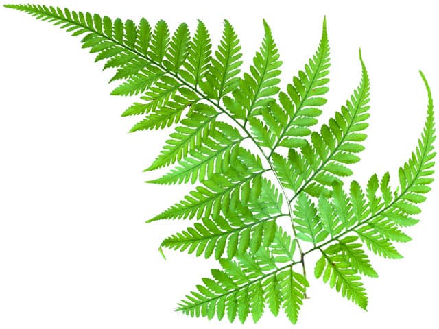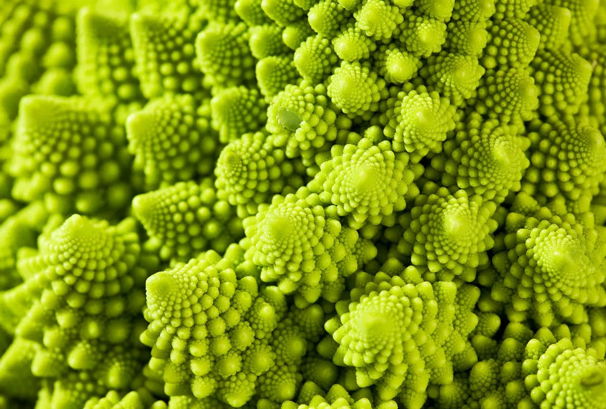:::Initially, these appear like highly complex shapes – but when you look closer, you might notice that they both follow a relatively simple pattern: all the individual parts of the plants look the same as the entire plant, just smaller. The same pattern is repeated over and over again, at smaller scales. In mathematics, we call this property **self-similarity**, and shapes that have it are called **fractals.**## **What is Fractal**?A [**fractal**](https://abhirup-moitra-mathstat.netlify.app/fractalR/fractal-harmony/) is a geometric shape that has a *fractional dimension*. Many famous fractals are *self-similar*, which means that they consist of smaller copies of themselves. Fractals contain patterns at every level of magnification, and they can be created by repeating a procedure or iterating an equation infinitely many times. They are some of the most beautiful and bizarre objects in all of mathematics. To create our fractals, we have to start with a simple pattern and then repeat it over and over again, at smaller scales.## **Fractals on Plant**### **Fractal Canopy**One of the simplest patterns might be a line segment, with two more segments branching off one end. If we repeat this pattern, both of these segments will also have two more branches at their ends.::: {layout-nrow="2"}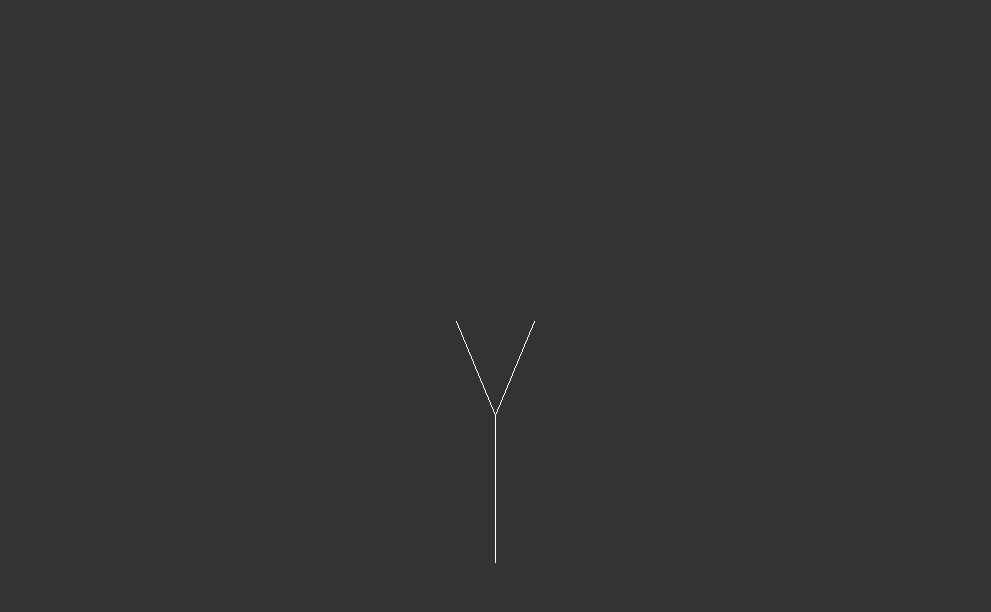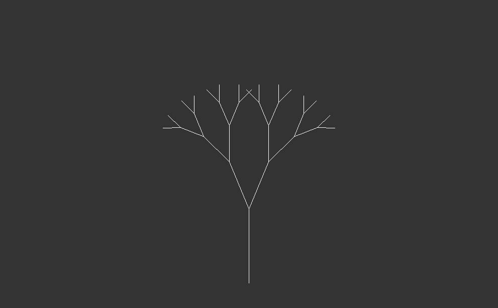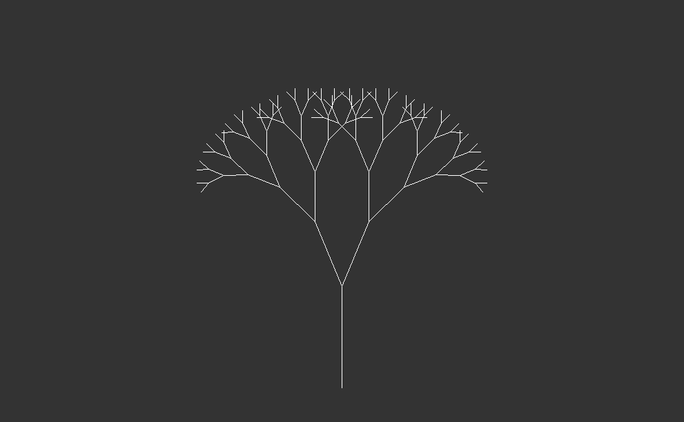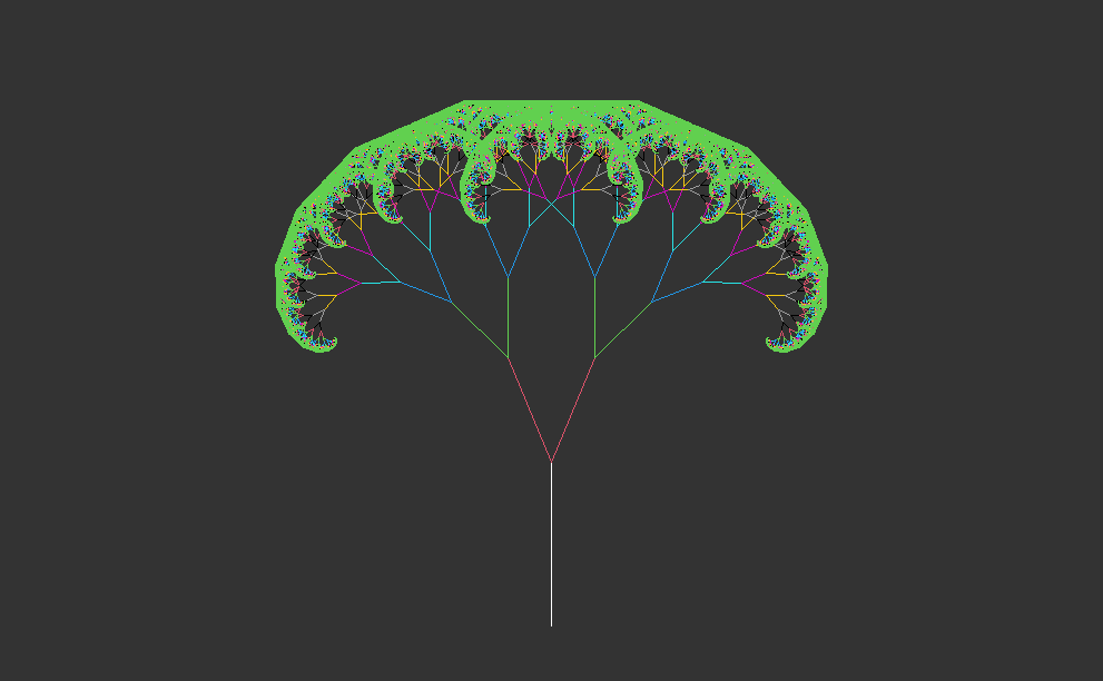:::Starting with a single trunk, they grow into larger branches, which then split into smaller branches recursively. This process repeats indefinitely, creating increasingly complex patterns.In nature, both trees and **forest canopies** follow similar rules to grow. It’s like when you see a big tree in the woods, and then you notice that its smaller branches look just like the big ones. This happens again and again, making the whole forest look like a big version of one small part. It’s like nature’s way of using the same pattern over and over to create something big and beautiful. ```{r,eval=FALSE}#---------------Fractal Canopy-------------------------------------------library(R6)library(ggplot2)library(uuid)options(stringsAsFactors = FALSE)branch_base = R6Class('branch_base', public = list( start_x = NA_integer_, start_y = NA_integer_, end_x = NA_integer_, end_y = NA_integer_, type = NA_character_, id = NA_character_, branch_color = NA_character_ ), # public active = list( df = function() { x = c(self$start_x, self$end_x) y = c(self$start_y, self$end_y) data.frame(x = x, y = y, type = self$type, id = self$id, branch_color = self$branch_color) } ) # active ) # branch_basetrunk = R6Class('trunk', inherit = branch_base, public = list( initialize = function(len = 10, branch_color = '#000000') { self$start_x = 0 self$start_y = 0 self$end_x = 0 self$end_y = len self$type = 'trunk' self$branch_color = branch_color self$id = uuid::UUIDgenerate() } ) # public ) # trunkbranch = R6Class('branch', inherit = branch_base, public = list( initialize = function(x, y, len = 5, theta = 45, type = NA_character_, branch_color='#000000') { dy = sin(theta) * len dx = cos(theta) * len self$start_x = x self$start_y = y self$end_x = x + dx self$end_y = y + dy self$type = type self$id = uuid::UUIDgenerate() self$branch_color = branch_color } ) # public ) # branchfractal_tree = R6Class('fractal_tree', public = list( delta_angle = NA_real_, len_decay = NA_real_, min_len = NA_real_, branches = data.frame(), branch_left_color = NA_character_, branch_right_color = NA_character_, initialize = function(trunk_len = 10, delta_angle = pi / 8, len_decay = 0.7, min_len = 0.25, trunk_color = '#000000', branch_left_color = '#000000', branch_right_color = '#adadad') { self$delta_angle = delta_angle self$len_decay = len_decay self$min_len = min_len self$branch_left_color = branch_left_color self$branch_right_color = branch_right_color self$branches = trunk$new(trunk_len, trunk_color)$df private$grow_branches(0, trunk_len, len = trunk_len * len_decay, angle_in = pi / 2) }, # initialize plot = function() { ggplot(tree$branches, aes(x, y, group = id, color=branch_color)) + geom_line() + geom_point(color = 'darkgreen', size=0.5) + scale_color_identity() + guides(color = FALSE, linetype = FALSE) + theme_void() } ), # public private = list( grow_branches = function(start_x, start_y, len = 1, angle_in = pi / 2, parent_type = NA, parent_color = NA) { if (len >= self$min_len) { l_type = if (!is.na(parent_type)) parent_type else 'left' r_type = if (!is.na(parent_type)) parent_type else 'right' l_color = if (!is.na(parent_color))parent_color else self$branch_left_color r_color = if (!is.na(parent_color)) parent_color else self$branch_right_color branch_left = branch$new(start_x, start_y, len, angle_in + self$delta_angle, l_type, l_color) branch_right = branch$new(start_x, start_y, len, angle_in - self$delta_angle, r_type, r_color) self$branches = rbind(self$branches, branch_left$df, branch_right$df) private$grow_branches(branch_left$end_x, branch_left$end_y, angle_in = angle_in + self$delta_angle, len = len * self$len_decay, parent_type = branch_left$type, parent_color = branch_left$branch_color) private$grow_branches(branch_right$end_x, branch_right$end_y, angle_in = angle_in - self$delta_angle,len = len * self$len_decay, parent_type = branch_right$type, parent_color = branch_right$branch_color) } } # grow_branches ) # private ) # fractal_treetree = fractal_tree$new()tree$plot()#__________________________________________________________________________________# Create/animate fractal trees at various angles for branch splitslibrary(gganimate)library(ggplot2)library(uuid)options(stringsAsFactors = FALSE)# create line segment from (0, 0) to (0, len) to be trunk of fractal treecreate_trunk = function(len = 1) { end_point = c(0, len) trunk_df = data.frame(x=c(0, 0), y=end_point, id=uuid::UUIDgenerate()) return(list(df=trunk_df, end_point=end_point))}# creates end point of line segment to satisfy length and# angle inputs from given start coordgen_end_point = function(xy, len = 5, theta = 45) { dy = sin(theta) * len dx = cos(theta) * len newx = xy[1] + dx newy = xy[2] + dy return(c(newx, newy))}# create a single branch of fractal tree# returns branch endpoint coords and a plotly line shape to represent branchbranch = function(xy, angle_in, delta_angle, len) { end_point = gen_end_point(xy, len = len, theta = angle_in + delta_angle) branch_df = as.data.frame(rbind(xy, end_point)) rownames(branch_df) = NULL names(branch_df) = c('x', 'y') branch_df$id = uuid::UUIDgenerate() return(list(df=branch_df, end_point=end_point))}# helper function to aggregate branch objects into single branch objectcollect_branches = function(branch1, branch2) { return(list(df=rbind(branch1$df, branch2$df)))}# recursively create fractal tree branchescreate_branches = function(xy, angle_in = pi / 2, delta_angle = pi / 8, len = 1, min_len = 0.01, len_decay = 0.2) { if (len < min_len) { return(NULL) } else { branch_left = branch(xy, angle_in, delta_angle, len) subranches_left = create_branches(branch_left$end_point, angle_in = angle_in + delta_angle, delta_angle = delta_angle, len = len * len_decay, min_len = min_len, len_decay = len_decay) branches_left = collect_branches(branch_left, subranches_left) branch_right = branch(xy, angle_in, -delta_angle, len) subranches_right = create_branches(branch_right$end_point, angle_in = angle_in - delta_angle, delta_angle = delta_angle, len = len * len_decay, min_len = min_len, len_decay = len_decay) branches_right = collect_branches(branch_right, subranches_right) return(collect_branches(branches_left, branches_right)) }}# create full fractal treecreate_fractal_tree_df = function(trunk_len=10, delta_angle = pi / 8, len_decay=0.7, min_len=0.25) { trunk = create_trunk(trunk_len) branches = create_branches(trunk$end_point, delta_angle = delta_angle, len = trunk_len * len_decay, min_len = min_len, len_decay = len_decay) tree = collect_branches(trunk, branches)$df return(tree)}# create a series of trees from a sequence of angles for branch splitscreate_fractal_tree_seq = function(trunk_len=10, angle_seq=seq(0, pi, pi/16), len_decay=0.7, min_len=0.25) { tree_list = lapply(seq_along(angle_seq), function(i) { tree_i = create_fractal_tree_df(trunk_len, angle_seq[i], len_decay, min_len) tree_i$frame = i tree_i$angle = angle_seq[i] return(tree_i) }) return(do.call(rbind, tree_list))}# create/animate a series of trees using gganimateanimate_fractal_tree = function(trunk_len=10, angle_seq=seq(0, pi, pi/16), len_decay=0.7, min_len=0.25, filename=NULL) { trees = create_fractal_tree_seq(trunk_len, angle_seq, len_decay, min_len) ggplot(trees, aes(x, y, group=id)) + geom_line() + geom_point(size=.2, aes(color=angle)) + scale_color_gradientn(colours = rainbow(5)) + guides(color=FALSE) + theme_void() + transition_manual(frame)}# example usageanimate_fractal_tree(trunk_len=10, angle_seq=seq(0, 2 * pi - pi / 32, pi/32), len_decay=0.7, min_len=.25)```::: {layout-ncol="2"}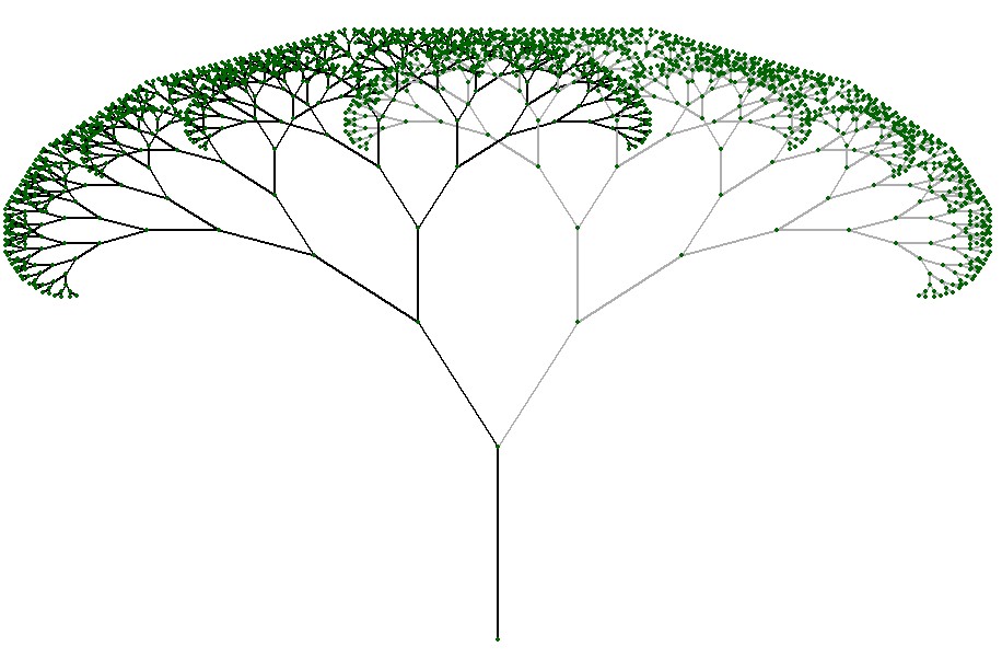{width="350"}:::Branching structures offer a fascinating canvas for exploring the diverse array of patterns found in nature. Depending on the arrangement and orientation of the branches, a myriad of captivating patterns can emerge. Look upward, and you may observe a canopy resembling a lush forest, with branches intertwining and spreading outwards to create a mesmerizing network of shapes and shadows.### Barnsley **Fern**Alternatively, cast your gaze downward, and you might encounter intricate patterns reminiscent of fern fronds, with delicate tendrils spiraling gracefully toward the ground. Here, amidst the forest floor, lies another realm of fractal beauty—the intricate carpet of mosses, lichens, and fungi. Like miniature landscapes writ small, these organisms form a tapestry of textures and shapes that mirror the fractal patterns found in the canopy above.```{r,eval=FALSE}## pBarnsleyFern(fn, n, clr, ttl, psz=600): Plot Barnsley fern fractal.## Where: fn - file name; n - number of dots; clr - color; ttl - plot title;## psz - picture size.## 7/27/16 aevpBarnsleyFern <- function(fn, n, clr, ttl, psz=600) { cat(" *** START:", date(), "n=", n, "clr=", clr, "psz=", psz, "\n"); cat(" *** File name -", fn, "\n"); pf = paste0(fn,".png"); # pf - plot file name A1 <- matrix(c(0,0,0,0.16,0.85,-0.04,0.04,0.85,0.2,0.23,-0.26,0.22,-0.15,0.26,0.28,0.24), ncol=4, nrow=4, byrow=TRUE); A2 <- matrix(c(0,0,0,1.6,0,1.6,0,0.44), ncol=2, nrow=4, byrow=TRUE); P <- c(.01,.85,.07,.07); # Creating matrices M1 and M2. M1=vector("list", 4); M2 = vector("list", 4); for (i in 1:4) { M1[[i]] <- matrix(c(A1[i,1:4]), nrow=2); M2[[i]] <- matrix(c(A2[i, 1:2]), nrow=2); } x <- numeric(n); y <- numeric(n); x[1] <- y[1] <- 0; for (i in 1:(n-1)) { k <- sample(1:4, prob=P, size=1); M <- as.matrix(M1[[k]]); z <- M%*%c(x[i],y[i]) + M2[[k]]; x[i+1] <- z[1]; y[i+1] <- z[2]; } plot(x, y, main=ttl, axes=FALSE, xlab="", ylab="", col=clr, cex=0.1); # Writing png-file dev.copy(png, filename=pf,width=psz,height=psz); # Cleaning dev.off(); graphics.off(); cat(" *** END:",date(),"\n");}## Executing:pBarnsleyFern("BarnsleyFernR", 100000, "dark green", "Barnsley Fern Fractal", psz=600)library(grid)A=vector('list',4)A[[1]]=matrix(c(0,0,0,0.18),nrow=2)A[[2]]=matrix(c(0.85,-0.04,0.04,0.85),nrow=2)A[[3]]=matrix(c(0.2,0.23,-0.26,0.22),nrow=2)A[[4]]=matrix(c(-0.15,0.36,0.28,0.24),nrow=2)b=vector('list',4)b[[1]]=matrix(c(0,0))b[[2]]=matrix(c(0,1.6))b[[3]]=matrix(c(0,1.6))b[[4]]=matrix(c(0,0.54))n <- 500000x <- numeric(n)y <- numeric(n)x[1] <- y[1] <- 0for (i in 1:(n-1)) {trans <- sample(1:4, prob=c(.02, .9, .09, .08), size=1)xy <- A[[trans]]%*%c(x[i],y[i]) + b[[trans]]x[i+1] <- xy[1]y[i+1] <- xy[2]}plot(y,x,col= 'darkgreen',cex=0.1)```::: {layout-ncol="2"}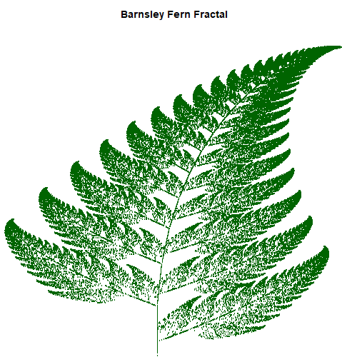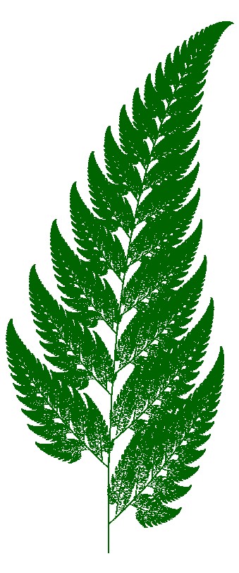{width="260"}:::Perhaps in the mosses that we find the true embodiment of fractal beauty. With their lush carpets and intricate branching patterns, mosses create miniature landscapes that echo the grandeur of the forest above. Each tiny leaflet follows the same basic form, repeating and branching outwards in a self-similar pattern that extends from the smallest scale to the largest.### **Pythagoras Tree**Moreover, an intricate **Pythagoras Tree** may emerge, showcasing the mathematical beauty inherent in branching structures. As you delve deeper into this exploration, you'll uncover a treasure trove of patterns waiting to be discovered. In this way, the forest floor becomes a canvas upon which nature paints its masterpiece—a testament to the elegance and complexity of fractal geometry. As you wander through this enchanted realm, take a moment to marvel at the intricate patterns that surround you, and you'll discover a world of wonder hidden in plain sight.```{r,eval=FALSE}## Recursive PT plottingpythtree <- function(ax,ay,bx,by,d) { if(d<0) {return()}; clr="darkgreen"; dx=bx-ax; dy=ay-by; x3=bx-dy; y3=by-dx; x4=ax-dy; y4=ay-dx; x5=x4+(dx-dy)/2; y5=y4-(dx+dy)/2; segments(ax,-ay,bx,-by, col=clr); segments(bx,-by,x3,-y3, col=clr); segments(x3,-y3,x4,-y4, col=clr); segments(x4,-y4,ax,-ay, col=clr); pythtree(x4,y4,x5,y5,d-1); pythtree(x5,y5,x3,y3,d-1);}## Plotting Pythagoras Tree. aev 3/27/17## x1,y1,x2,y2 - starting position## ord - order/depth, fn - file name, ttl - plot title.pPythagorasT <- function(x1, y1,x2, y2, ord, fn="", ttl="") { cat(" *** START PYTHT:", date(), "\n"); m=640; i=j=k=m1=m-2; x=y=d=dm=0; if(fn=="") {pf=paste0("PYTHTR", ord, ".png")} else {pf=paste0(fn, ".png")}; if(ttl=="") {ttl=paste0("Pythagoras tree, order - ", ord)}; cat(" *** Plot file -", pf, "title:", ttl, "\n"); plot(NA, xlim=c(0,m), ylim=c(-m,0), xlab="", ylab="", main=ttl); pythtree(x1,y1, x2,y2, ord); dev.copy(png, filename=pf, width=m, height=m); dev.off(); graphics.off(); cat(" *** END PYTHT:",date(),"\n");}## Executing:pPythagorasT(275,500,375,500,10) pPythagorasT(275,500,375,500,12)pPythagorasT(275,500,375,500,15)pPythagorasT(275,500,375,500,17)```::: {layout-nrow="2"}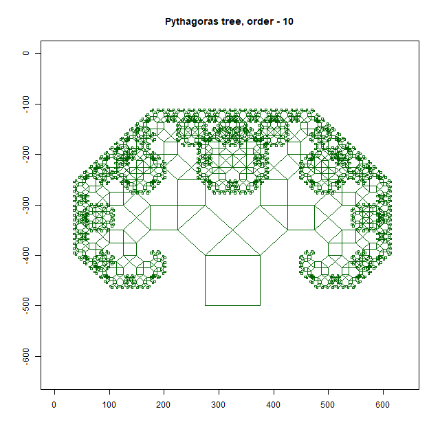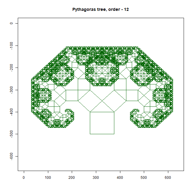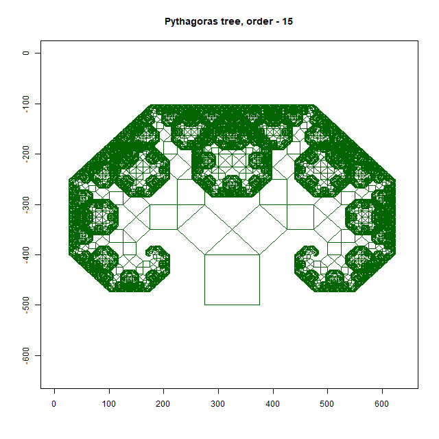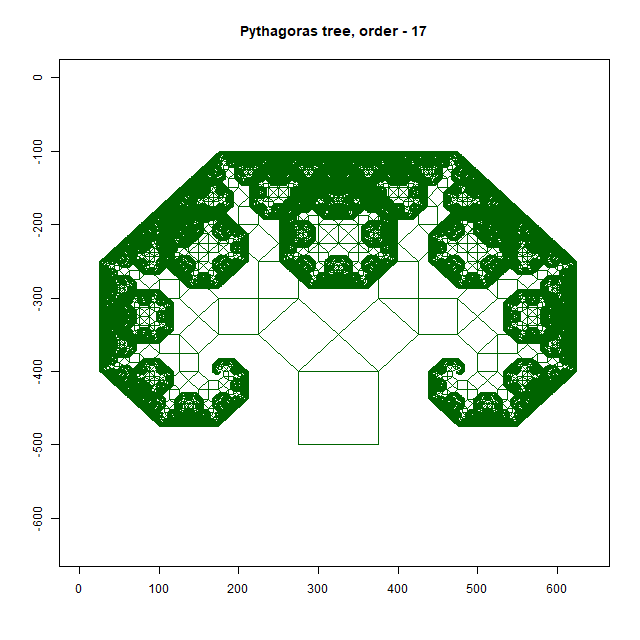:::## Geometric FractalsIn the vast tapestry of nature's complexity, there exists a fascinating realm of geometric fractals, where seemingly simple shapes give rise to intricate and mesmerizing patterns. These fractals, characterized by self-similarity and recursive structures, offer a glimpse into the underlying order and beauty of the natural world.At the heart of geometric fractals lies a concept known as self-similarity, where the structure of an object repeats itself at different scales. This property, evident in fractals like the *Sierpinski Triangle, Sierpinski Carpet, and Sierpinski Arrowhead* (The Arrowhead Curve is a curve that traces out the same shape as the Sierpinski Triangle.) allows for the creation of stunningly detailed patterns that exhibit complexity on both macroscopic and microscopic levels. Geometric fractals not only captivate the imagination but also have practical applications in various fields, including computer graphics, image compression, and even the study of natural phenomena like coastlines and clouds. By unraveling the secrets of these fascinating structures, scientists and mathematicians continue to uncover new insights into the underlying principles that govern our universe.In the realm of science, the study of geometric fractals serves as a reminder of the inherent order and complexity that permeates the natural world. From the intricate patterns of snowflakes to the sprawling landscapes of coastlines, fractals offer a window into the hidden symmetries and patterns that shape our reality. As we delve deeper into the mysteries of geometric fractals, we embark on a journey of discovery that unveils the wondrous beauty of nature's infinite complexity.There are many ways to generate geometric fractals. First, we will begin with the process of repeated removal and an exploration of the **Sierpinski Triangle**.### **Sierpinski Triangle**#### **Introduction**The Sierpinski triangle, named after the Polish mathematician [Wacław Sierpiński](https://en.wikipedia.org/wiki/Wac%C5%82aw_Sierpi%C5%84ski), is one of the most iconic geometric fractals. This fractal is formed through a recursive process of subdividing a triangle into smaller triangles and removing the central triangle at each iteration. The resulting pattern is characterized by intricate triangular shapes nested within one another, demonstrating the mesmerizing beauty of self-similarity.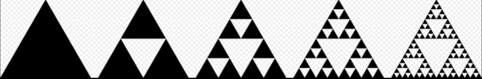{fig-align="center"}#### **Origin**At its core, the Sierpinski triangle is a self-similar fractal, comprised of an equilateral triangle with smaller equilateral triangles recursively removed from its remaining area. This recursive removal process creates a fascinating visual effect, wherein the final shape consists of three identical copies of itself, each composed of even smaller copies of the entire triangle. This property allows for an endless zooming-in process, with patterns and shapes continuously repeating at ever-smaller scales.```{r,eval=FALSE}serpenski2 <- function(tmp.depth) {## An X or Y means move forward 1 unit.## A "+" or a "-" means turn right of left 60 degrees.path <- c("Y","+","X","+","Y")X.g <- c("Y","+","X","+","Y")Y.g <- c("X","-","Y","-","X")depth<-tmp.depth - 1if(depth>0) for(j in 1:depth) {(ruler <- length(path))path.grow <- character(ruler*3+2)tmp.which <- which(path %in% c("+","-"))path.grow[3*tmp.which] <- path[tmp.which]tmp.which <- which(path == "Y")path.grow[eval(parse(text=paste0("c(",paste(tmp.which*3-2,":",tmp.which*3+2,collapse=','),")")))]<-rep(Y.g,length(tmp.which))tmp.which <- which(path == "X")path.grow[eval(parse(text=paste0("c(",paste(tmp.which*3-2,":",tmp.which*3+2,collapse=','),")")))]<-rep(X.g,length(tmp.which))path <- path.grow}## From 'path' create the x and y coordinates to plot.x<-c(0,cumsum(sin(c(0,cumsum(ifelse(path[seq(2,length(path),2)]=="+", 1,-1))*pi/3))))y<-c(0,cumsum(cos(c(0,cumsum(ifelse(path[seq(2,length(path),2)]=="+", 1,-1))*pi/3))))## plot!!plot(x,y,type='l',main="Serpenski Triangle")mtext(paste0("Depth = ",tmp.depth),4)}serpenski2(1)serpenski2(2)serpenski2(3)serpenski2(4)serpenski2(5)serpenski2(6)serpenski2(7)serpenski2(8)serpenski2(9)serpenski2(10)serpenski2(12)```#### **Construction**The construction of the Sierpinski triangle follows a systematic progression. Starting with a simple equilateral triangle, the first step involves removing the middle triangle, leaving behind three black triangles surrounding a central white triangle (iteration 1). This process is then repeated at a smaller scale, removing the middle third of each of the three remaining triangles, resulting in the second iteration with nine smaller black triangles. The number of smallest triangles triples with each iteration, yielding 27 triangles in the third iteration and 81 triangles in the fourth iteration. This tripling pattern continues indefinitely, and the number of triangles, denoted as $T$, can be expressed as $T=3^n$, where $n$ represents the iteration level.::: {layout-ncol="2"}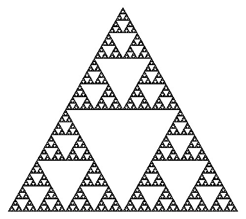{width="368"}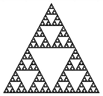:::Sierpinski triangle demonstrates the elegance of fractal geometry and finds applications across various fields, from mathematics to computer science and even art.### **The Sierpinski Carpet**#### **Introduction**The Sierpinski Carpet, a captivating fractal pattern, was introduced by the Polish mathematician Wacław Sierpiński in 1916. This fractal, also known as the Sierpiński square or the Sierpiński sponge in three dimensions, exhibits intricate self-similarity and has captured the imagination of mathematicians, artists, and enthusiasts alike.#### **Origin**Wacław Sierpiński conceived the Sierpinski Carpet as a natural extension of his work on fractals, following his exploration of the Sierpinski triangle. The carpet's inception marked a significant advancement in the understanding of fractal geometry and its applications across diverse fields.#### **Construction**The construction of the Sierpinski Carpet follows a straightforward iterative process that yields strikingly complex results. Begin with a square divided into nine equal smaller squares arranged in a 3x3 grid. Remove the central square, leaving behind eight smaller squares. Repeat this process for each remaining square indefinitely. Through this recursive procedure, the Sierpinski Carpet emerges—a geometric wonder characterized by an infinitely repeating pattern of voids within a larger square.The construction of the Sierpinski Carpet exemplifies the recursive nature of fractals, where simple rules repeated over and over again produce intricate and mesmerizing patterns. Despite its seemingly straightforward construction, the Sierpinski Carpet possesses remarkable properties, such as infinite perimeter and zero area, challenging conventional notions of geometry and dimensionality.```{r,eval=FALSE}IterateCarpet <- function(A){B <- cbind(A,A,A);C <- cbind(A,0*A,A);D <- rbind(B,C,B);return(D);}S <- matrix(1,1,1);for (i in 1:5) S <- IterateCarpet(S);image(S,col=c(0, 12), axes=FALSE);library(ggplot2)library(grid)SierpinskiCarpet <- function(k){ Iterate <- function(M){ A <- cbind(M,M,M); B <- cbind(M,0*M,M); return(rbind(A,B,A)) } M <- as.matrix(1) for (i in 1:k) M <- Iterate(M); n <- dim(M)[1] X <- numeric(n) Y <- numeric(n) I <- numeric(n) for (i in 1:n) for (j in 1:n){ X[i + (j-1)*n] <- i; Y[i + (j-1)*n] <- j; I[i + (j-1)*n] <- M[i,j]; } DATA <- data.frame(X,Y,I) p <- ggplot(DATA,aes(x=X,y=Y,fill=I)) p <- p + geom_tile() + theme_bw() + scale_fill_gradient(high=rgb(0,0,0),low=rgb(1,1,1)) p <-p+ theme(legend.position=0) + theme(panel.grid = element_blank()) p <- p+ theme(axis.text = element_blank()) + theme(axis.ticks = element_blank()) p <- p+ theme(axis.title = element_blank()) + theme(panel.border = element_blank()); return(p)}A <- viewport(0.25,0.75,0.45,0.45)B <- viewport(0.75,0.75,0.45,0.45)C <- viewport(0.25,0.25,0.45,0.45)D <- viewport(0.75,0.25,0.45,0.45)print(SierpinskiCarpet(1),vp=A)print(SierpinskiCarpet(2),vp=B)print(SierpinskiCarpet(3),vp=C)print(SierpinskiCarpet(4),vp=D)print(SierpinskiCarpet(6),vp=D)print(SierpinskiCarpet(7),vp=D)```::: {layout-nrow="2"}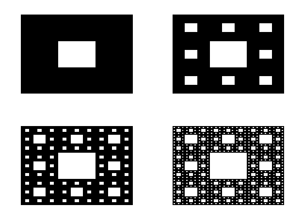{width="448"}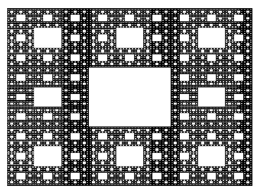{width="414"}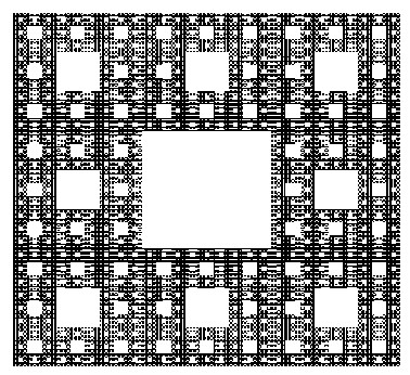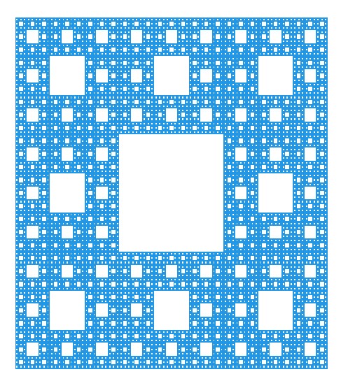{width="317"}:::Over the years, the Sierpinski Carpet has found applications in diverse fields, including mathematics, computer science, and art. Its elegant simplicity coupled with its mesmerizing complexity continues to inspire exploration and creativity, making it a timeless masterpiece in the realm of fractal geometry.### **The Koch Snowflake**#### **Introduction**In the realm of mathematical beauty, few patterns captivate the imagination quite like the **Koch snowflake.** This intricate fractal, named after the Swedish mathematician [Helge von Koch](https://en.wikipedia.org/wiki/Niels_Fabian_Helge_von_Koch), showcases the mesmerizing synergy between simplicity and complexity found in nature's design. As we embark on our journey to unravel the secrets of this geometric wonder, we delve into its origins, construction, and significance in both mathematics and the natural world.#### **Origins**The story of the Koch snowflake begins in the early 20th century when *Helge von Koch* introduced the concept as a means to explore the notion of infinite perimeter within a finite area. In 1904, Koch presented his groundbreaking paper, "*On a Continuous Curve Without Tangents, Constructible from Elementary Geometry*," unveiling this remarkable fractal.#### **Construction**At its core, the Koch snowflake emerges from a deceptively simple iterative process. Start with an equilateral triangle, then replace the middle third of each line segment with two segments of equal length, forming a smaller equilateral triangle. Repeat this process infinitely for each remaining line segment, and behold—the Koch snowflake emerges in all its intricate glory. Despite its seemingly straightforward construction, the Koch snowflake possesses an infinite perimeter, yet encloses a finite area—an astounding paradox that showcases the beauty of fractal geometry.## **The Algorithmic Approach & Visualization:The Koch Curve to Koch Snowflake**The Koch curve starts from a straight line which is broken into three equally long pieces. Next, two new lines, which are just as long as one the three pieces, are added on top of the initial line. Together with the center piece they form an equilateral triangle. Lastly, the center piece is removed from the initial line. These steps are then recursively applied to every line in the curve. Here is what that looks like after zero, one, two and three iterations:```{r,eval=FALSE}# function to create empty canvasemptyCanvas <- function(xlim, ylim, bg="gray20") { par(mar=rep(1,4), bg=bg) plot(1, type="n", bty="n", xlab="", ylab="", xaxt="n", yaxt="n", xlim=xlim, ylim=ylim)}# example#emptyCanvas(xlim=c(0,1), ylim=c(0,1))# function to draw a single linedrawLine <- function(line, col="white", lwd=1) { segments(x0=line[1], y0=line[2], x1=line[3], y1=line[4], col=col, lwd=lwd)}# wrapper around "drawLine" to draw entire objectsdrawObject <- function(object, col="white", lwd=1) { invisible(apply(object, 1, drawLine, col=col, lwd=lwd))}# exampleline1 = c(0,0,1,1)line2 = c(-3,4,-2,-4)line3 = c(1,-3,4,3)mat = matrix(c(line1,line2,line3), byrow=T, nrow=3)# function to add a new line to an existing onenewLine <- function(line, angle, reduce=1) { x0 <- line[1] y0 <- line[2] x1 <- line[3] y1 <- line[4] dx <- unname(x1-x0) # change in x direction dy <- unname(y1-y0) # change in y direction l <- sqrt(dx^2 + dy^2) # length of the line theta <- atan(dy/dx) * 180 / pi # angle between line and origin rad <- (angle+theta) * pi / 180 # (theta + new angle) in radians coeff <- sign(theta)*sign(dy) # coefficient of direction if(coeff == 0) coeff <- -1 x2 <- x0 + coeff*l*cos(rad)*reduce + dx # new x location y2 <- y0 + coeff*l*sin(rad)*reduce + dy # new y location return(c(x1,y1,x2,y2))}a = c(-1.2,1,1.2,1)b = newLine(a, angle=-90, reduce=1)c = newLine(b, angle=45, reduce=.72)d = newLine(c, angle=90, reduce=1)e = newLine(d, angle=45, reduce=1.4)# draw linesemptyCanvas(xlim=c(-5,5), ylim=c(0,5))drawLine(a, lwd=3, col="white")drawLine(b, lwd=3, col="orange")drawLine(c, lwd=3, col="cyan")drawLine(d, lwd=3, col="firebrick")drawLine(e, lwd=3, col="limegreen")# function to run next iteration based on "ifun()"iterate <- function(object, ifun, ...) { linesList <- vector("list",0) for(i in 1:nrow(object)) { old_line <- matrix(object[i,], nrow=1) new_line <- ifun(old_line, ...) linesList[[length(linesList)+1]] <- new_line } new_object <- do.call(rbind, linesList) return(new_object)}# iterator function: koch curvekoch <- function(line0) { # new triangle (starting at right) line1 <- newLine(line0, angle=180, reduce=1/3) line2 <- newLine(line1, angle=-60, reduce=1) line3 <- newLine(line2, angle=120, reduce=1) line4 <- newLine(line3, angle=-60, reduce=1) # reorder lines (to start at left) line1 <- line1[c(3,4,1,2)] line2 <- line2[c(3,4,1,2)] line3 <- line3[c(3,4,1,2)] line4 <- line4[c(3,4,1,2)] # store in matrix and return mat <- matrix(c(line4,line3,line2,line1), byrow=T, ncol=4) return(mat)}# example: Koch curve (after one iterations)fractal <- matrix(c(10,0,20,1e-9), nrow=1)for(i in 1:1) fractal <- iterate(fractal, ifun=koch)emptyCanvas(xlim=c(10,20), ylim=c(0,3))drawObject(fractal)# example: Koch curve (after two iterations)fractal <- matrix(c(10,0,20,1e-9), nrow=1)for(i in 1:2) fractal <- iterate(fractal, ifun=koch)emptyCanvas(xlim=c(10,20), ylim=c(0,3))drawObject(fractal)# example: Koch curve (after three iterations)fractal <- matrix(c(10,0,20,1e-9), nrow=1)for(i in 1:3) fractal <- iterate(fractal, ifun=koch)emptyCanvas(xlim=c(10,20), ylim=c(0,3))drawObject(fractal)# example: Koch curve (after four iterations)fractal <- matrix(c(10,0,20,1e-9), nrow=1)for(i in 1:4) fractal <- iterate(fractal, ifun=koch)emptyCanvas(xlim=c(10,20), ylim=c(0,3))drawObject(fractal)# example: Koch curve (after five iterations)fractal <- matrix(c(10,0,20,1e-9), nrow=1)for(i in 1:5) fractal <- iterate(fractal, ifun=koch)emptyCanvas(xlim=c(10,20), ylim=c(0,3))drawObject(fractal)# example: Koch curve (after six iterations)fractal <- matrix(c(10,0,20,1e-9), nrow=1)for(i in 1:6) fractal <- iterate(fractal, ifun=koch)emptyCanvas(xlim=c(10,20), ylim=c(0,3))drawObject(fractal)```::: {layout-nrow="2"}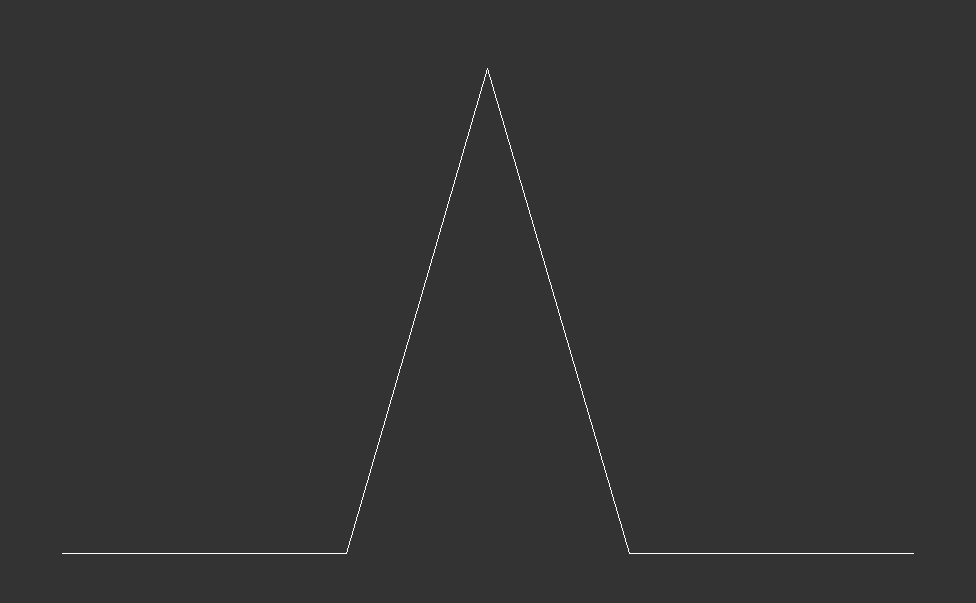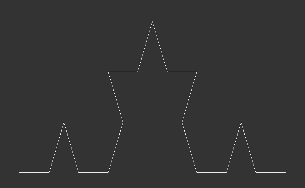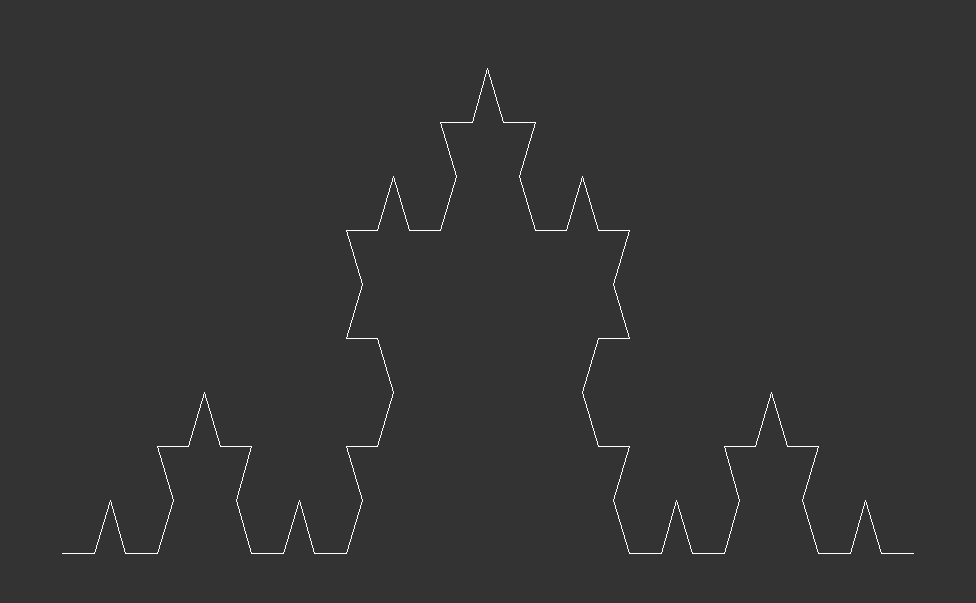:::In terms of programming the Koch curve, we start from the end point of the initial line and make an $180^{0}$ turn. Then we use the fact that all angles of an equilateral triangle have $60^{0}$ . This means we first turn by negative 60 degrees, then by 120 degrees and finally another negative $60^{0}$ to reach the initial start point. For the first of the four line segments, we set `reduce=1/3`, thereafter we set `reduce=1`, as we do not need to shorten the segments any further.::: {layout-ncol="2"}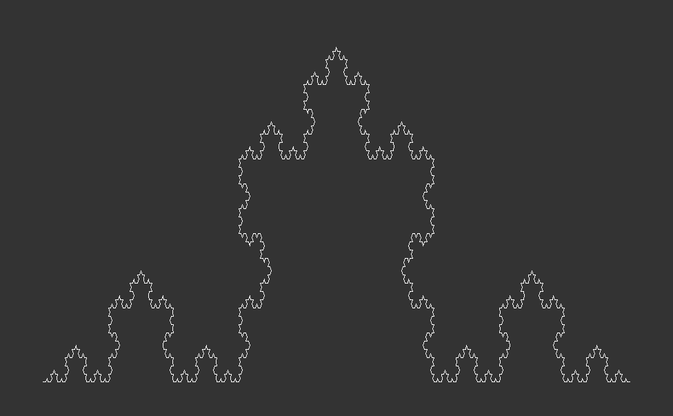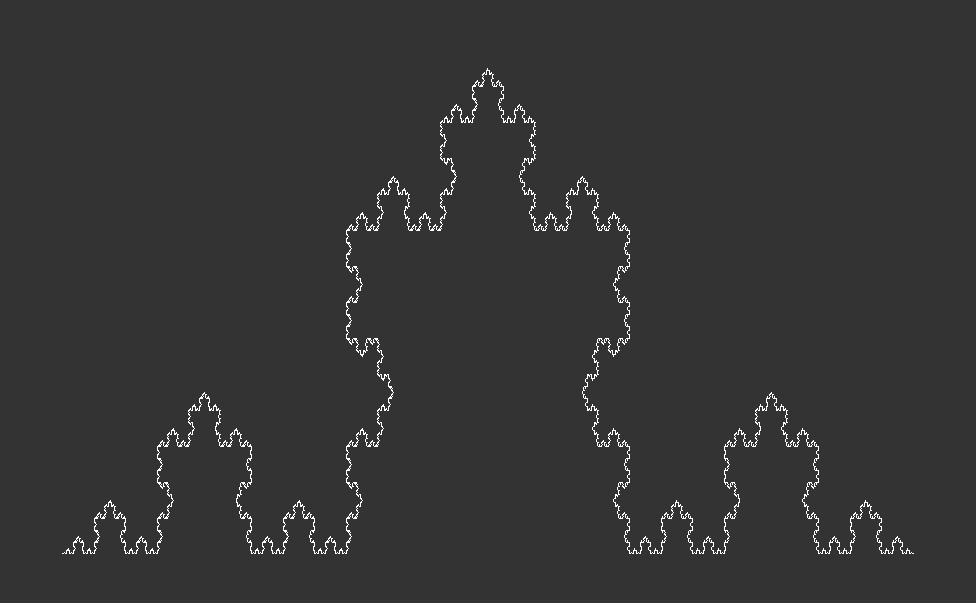:::As this recursive process continues indefinitely, each iteration adds more detail, creating a snowflake with an infinitely complex, self-similar pattern that extends infinitely into both the micro and macroscopic scales.```{r,eval=FALSE}# Koch snowflake (after six iterations)A <- c(0,1e-9)B <- c(3,5)C <- c(6,0)fractal <- matrix(c(A,B,B,C,C,A), nrow=3, byrow=T)for(i in 1:6) fractal <- iterate(fractal, ifun=koch)emptyCanvas(xlim=c(-2,8), ylim=c(-2,5))drawObject(fractal)```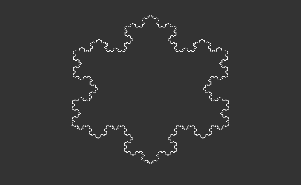{fig-align="center" width="662"}Notice that we set some coordinates to `1e9` instead of exactly $0$. This is to avoid some corner cases but does not make any difference at all when drawing the fractal images.# **Conclusion**Geometric fractals not only captivate the imagination but also have practical applications in various fields, including computer graphics, image compression, and even the study of natural phenomena like coastlines and clouds. By unraveling the secrets of these fascinating structures, scientists and mathematicians continue to uncover new insights into the underlying principles that govern our universe.In the realm of science, the study of geometric fractals serves as a reminder of the inherent order and complexity that permeates the natural world. From the intricate patterns of snowflakes to the sprawling landscapes of coastlines, fractals offer a window into the hidden symmetries and patterns that shape our reality. As we delve deeper into the mysteries of geometric fractals, we embark on a journey of discovery that unveils the wondrous beauty of nature's infinite complexity.# **Footnotes**- [**Fractal Garden : An Exhibition Of Mathematical Beauty**](https://www.fractal.garden/)- [**The Mathematical Playground**](https://mathigon.org/course/fractals/introduction)# **See Also**- [**Unraveling Nature’s Code: The Wonders of Fractal Geometry.**](https://abhirup-moitra-mathstat.netlify.app/fractalR/fractal-harmony/)- [**Analyzing Fractal Complexity.**](https://abhirup-moitra-mathstat.netlify.app/fractalR/mathematical-anlysis1/project-analysis.html)- [**The Fractal Flame Algorithm**](https://flam3.com/flame_draves.pdf)- [**Sierpiński triangle**](https://en.wikipedia.org/wiki/Sierpi%C5%84ski_triangle)- [**Chaos Game**](https://en.wikipedia.org/wiki/Chaos_game)- [**The Artistry of Growth**](https://abhirup-moitra-mathstat.netlify.app/fractalR/fractal-cannopies/)# **References**1. Shannon, Kathleen M.; Bardzell, Michael J. (November 2003). ["Patterns in Pascal's Triangle – with a Twist"](#0). *Convergence*. [Mathematical Association of America](#0 "Mathematical Association of America"). Retrieved 29 March 2015.2. Khovanova, Tanya; Nie, Eric; Puranik, Alok (2014), "The Sierpinski Triangle and the Ulam-Warburton Automaton", *Math Horizons*, **23** (1): 5–9, [arXiv](#0 "ArXiv (identifier)"):[1408.5937](#0), [doi](#0 "Doi (identifier)"):[10.4169/mathhorizons.23.1.5](#0), [S2CID](#0 "S2CID (identifier)") [125503155](#0)3. [""Sierpinski Gasket by Trema Removal""](http://www.cut-the-knot.org/triangle/Tremas.shtml).4. [**\^**](https://en.wikipedia.org/wiki/Sierpi%C5%84ski_triangle#cite_ref-2 "Jump up")[Michael Barnsley](https://en.wikipedia.org/wiki/Michael_Barnsley "Michael Barnsley"); et al. (2003), "V-variable fractals and superfractals", [arXiv](https://en.wikipedia.org/wiki/ArXiv_(identifier) "ArXiv (identifier)"):[math/0312314](https://arxiv.org/abs/math/0312314)5. Addison, Paul S. (1997). *Fractals and Chaos: An Illustrated Course*. Institute of Physics. p.19. [ISBN](#0 "ISBN (identifier)") [0-7503-0400-6](#0 "Special:BookSources/0-7503-0400-6").


