Analyzing Fractal Complexity

A Comprehensive Examination of Iterated Function Systems in Mathematical and Computational Sciences

Mathematics

R Programming

Author

Abhirup Moitra

Published

December 10, 2023

Nature builds up her refined and invisible architecture with a delicacy eluding our conception

Abstract

This research project delves into the domain of Iterated Function Systems (IFS), a mathematical framework within fractal geometry renowned for its capacity to produce intricate self-replicating patterns. The inquiry begins with an elucidation of the core components constituting an IFS, which involves a set of contraction mappings defined by mathematical functions. These functions, recognized for their contractive nature, iteratively transform points within a given space. Integral to the methodology of IFS is the integration of probabilities associated with each transformation, influencing the likelihood of selecting a specific function during the iterative process. Through the repetitive application of these functions and the infusion of randomness via probability weights, a sequence of points evolves, converging towards a fractal structure identified as the limit set. The study scrutinizes the convergence characteristics of IFS and the manifestation of self-similar patterns within the limit set. By examining the interplay between simplicity at the function level and the observed complexity at the macroscopic fractal level, the research underscores the captivating nature of IFS in generating visually compelling and intricate structures. Practical applications of IFS are explored, ranging from its role in computer graphics to applications in image compression techniques. The abstract nature of fractal patterns generated by IFS finds utility in diverse fields, offering a versatile tool for creating realistic, natural forms with self-repeating characteristics.

In conclusion, this exploration of Iterated Function Systems contributes to a deeper understanding of the mathematical principles underpinning fractal geometry and its applications in computer science. The study aims to underscore the significance of IFS as a powerful and flexible tool for generating complex, self-replicating structures with applications that extend across various domains of scientific inquiry and artistic expression.

1. Basic Formalism

1.1 Metric Space

A metric space is a mathematical structure that formalizes the concept of distance between points. It is a set equipped with a distance function (metric) that satisfies certain properties. The distance function assigns a non-negative real number to pairs of points in the set, representing the distance between those points.

Definition

A metric space consists of a set X and a metric $d: X \times X \to \mathbb{R}$ such that for any points $x,y,z$ in $X$, the following conditions, called the metric axioms, are satisfied:

Non-negativity: $d(x,y) \ge 0$ (distance is always non-negative).
Identity of indiscernibles: $d(x,y)=0$ if and only if $x=y$ (distinct points have positive distance).
Symmetry: $d(x,y)=d(y,x)$ (the distance between two points is the same regardless of the order).
Triangle inequality: $d(x,y)+d(y,z)≥d(x,z)$ (the direct route is always at least as short as any detour).

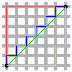
The plane (a set of points) can be equipped with different metrics. In the taxicab metric the red, yellow, and blue paths have the same length (12), and are all the shortest paths. In the Euclidean metric, the green path has length $6 \sqrt{2} \approx 8.49$, and is the unique shortest path, whereas the red, yellow, and blue paths still have a length of $12$.

1.2 Cauchy Sequence

A Cauchy sequence is a sequence whose elements become arbitrarily close to each other as the sequence progresses. More precisely, given any small positive distance, all excluding a finite number of elements of the sequence are less than that given distance from each other.

Definition

$\text{Let}\; (X,d)\; \text{be a metric space. Then}\; \{x_n\}_{n\ge1} \subseteq X\; \text{is called a Cauchy sequence if}\;$

\[ \forall \epsilon >0\ \exists N\in \mathbb{N}\ \forall m,n \ge N\;\;\ d(x_m,x_n) < \epsilon \]

1.3 Complete Metric Space

A metric space $(X,d)$ is called complete if every Cauchy sequence in that space converges to a limit that is also within the space.

This means that there are no “missing” points, and the space is closed under the limit operation for Cauchy sequences.

1.2 Iterated function

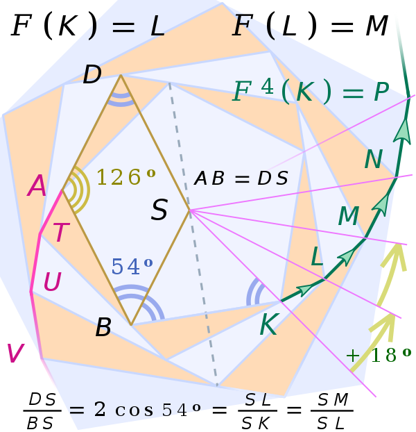
Let $X$ be a set and $f: X \to X$ be a function. Defining $f^n$ as the $n^\text{th}$ iterate of $f$. where $n$ is a non-negative integer. An iterated function is a function $X \to X$ (that is, a function from some set $X$ to itself) which is obtained by composing another function $f : X \to X$ with itself a certain number of times. The process of repeatedly applying the same function is called iteration. In this process, starting from some initial object, the result of applying a given function is fed again into the function as input, and this process is repeated.

\[ L = F(k) , M = F \circ F (k) = F^2(k) \]

For example on the image on the bottom

1.3 Iterated Function System(IFS)

Formally, an iterated function system(IFS) is a finite set of contraction mappings on a complete metric space. Symbolically,

\[ \{f_i : X \to X\ | \ i = 1,2,\ldots N\} \;\text{where}\; N \in \mathbb{N} \]

is an iterated function system if each $f_i$ is a contraction on the complete metric space $X$.

Hutchinson showed that, for the metric space $\mathbb{R}^n$, or more generally, for a complete metric space $X$, such a system of functions has a unique nonempty compact (closed and bounded) fixed set S.^[3] One way of constructing a fixed set is to start with an initial nonempty closed and bounded set S₀ and iterate the actions of the $fi$, taking $S_{n+1}$to to be the union of the images of $S_n$ under the $fi$; then taking $S$ to be the closure of the limit $\displaystyle\lim_{n \to \infty} S_n$. Symbolically, the unique fixed (nonempty compact) set $S \subseteq X$ has the property.

\[ S = \overline{\bigcup_{i=1}^N f_i(S)} \]

The set $S$ is thus the fixed set of the Hutchinson operator $F: 2^X \to 2^X$ defined $A \subseteq X$ via

\[F(A) =\overline{\bigcup_{i=1}^N f_i(A)} \]

The existence and uniqueness of $S$ is a consequence of the contraction mapping principle, as is the fact that

\[ \lim_{n \to \infty} F^n(A) = S \]

for any nonempty compact set $A$ in $X$. (For contractive IFS this convergence takes place even for any nonempty closed bounded set $A$). Random elements arbitrarily close to $S$may be obtained by the “chaos game,”

2. Contraction Mapping

An IFS involves a finite collection of functions. Each function in the set represents a transformation. Contractive maps, also known as contractions, are functions that bring points closer together. Specifically, a function $f$ is contractive if there exists a constant $0 \le k<1$ such that for any two points $x$ and $y$, the distance between $f(x)$ and $f(y)$ is less than $k$ times the distance between $x$ and $y$.

Definition

A contraction mapping, or contraction on a metric space $(M, d)$ is a function $f$ from $M$ to itself, with the property that there is some real number $0 \le k<1$ such that $\forall x,y \in M.$

\[ d(f(x), f(y)) \le k.d(x,y) \]

The smallest such value of $k$ is called the Lipschitz constant of $f$. Contractive maps are sometimes called Lipschitzian maps. If the above condition is instead satisfied for $k\le 1$, then the mapping is said to be a non-expansive map. More generally, the idea of a contractive mapping can be defined for maps between metric spaces. Thus, if $(M, d)$ and $(N, d')$ are two metric spaces, then $f : M \to N$ is a contractive mapping if there is a constant $0 \le k<1$ such that,

\[ d'(f(x), f(y)) \le k.d(x,y)\; \forall x,y \in M \]

Complete Metric Space,the functions in an IFS operate on a complete metric space. A metric space is a set equipped with a distance function (metric) that satisfies certain properties. Completeness implies that every Cauchy sequence in the space converges to a limit that is also within the space. The process of an Iterated Function System involves repeatedly applying these contractive maps to points in the metric space. This iteration can lead to interesting and complex patterns.

IFS is commonly used in the field of fractal geometry to generate self-replicating structures and patterns. One well-known example of an IFS is the construction of the Sierpinski triangle. Each function in the IFS is a contraction that transforms an equilateral triangle into a smaller equilateral triangle. Through iteration, this process generates the intricate Sierpinski triangle pattern.

3 Chaotic Realm

We have already come across the definition of an Iterated Function System(IFS) where each $f_i$ is a contraction on the complete metric space $X$. Each function $f_i$ is required to be a linear, or more generally an affine, transformation, and hence represented by a matrix. However, IFSs may also be built from non-linear functions, including projective transformations and Möbius transformations. The Fractal flame is an example of an IFS with nonlinear functions. The most common algorithm to compute IFS fractals is called the “chaos game”. It consists of picking a random point in the plane, and then iteratively applying one of the functions chosen at random from the function system to transform the point to get a next point. An alternative algorithm is to generate each possible sequence of functions up to a given maximum length, and then plot the results of applying each of these sequences of functions to an initial point or shape. Each of these algorithms provides a global construction that generates points distributed across the whole fractal. If a small area of the fractal is being drawn, many of these points will fall outside of the screen boundaries. This makes zooming into an IFS construction drawn in this manner impractical. Although the theory of IFS requires each function to be contractive, in practice software that implements IFS only requires that the whole system be contractive on average.

3.1 Chaos Game

The chaos game is an engaging and intuitive way to explore the fractal structures generated by IFS transformations. By iteratively applying random transformations to points in a space, you can observe the emergence of intricate and self-replicating patterns. In a research or coding project focused on IFS, incorporating the chaos game serves both educational and practical purposes. Here are some points you might consider emphasizing or exploring further.

3.2 Chaos Game For The Barnsley Fern

The fern is one of the basic examples of self-similar sets, i.e. it is a mathematically generated pattern that can be reproducible at any magnification or reduction. Barnsley’s 1988 book Fractals Everywhere is based on the course that he taught for undergraduate and graduate students in the School of Mathematics, Georgia Institute of Technology, called Fractal Geometry. After publishing the book, a second course was developed, called Fractal Measure Theory. Barnsley’s work has been a source of inspiration to graphic artists attempting to imitate nature with mathematical models. The fern code developed by Barnsley is an example of an iterated function system (IFS) to create a fractal. This follows from the collage theorem. He has used fractals to model a diverse range of phenomena in science and technology, but most specifically plant structures.

3.2.1 Collage Theorem

the collage theorem characterizes an iterated function system whose attractor is close, relative to the Hausdorff metric, to a given set. The IFS described is composed of contractions whose images, as a collage or union when mapping the given set, are arbitrarily close to the given set. It is typically used in fractal compression.

Statement

Let $\mathbb{X}$ be a complete metric space. Suppose $L$ is a nonempty, compact subset of $\mathbb{X}$ and let $\epsilon >0$ be given. Choose an iterated function system (IFS) $\{\mathbb{X};\ w_1, w_2, \ldots w_N\}$ with contractivity factor $s$ where $0 \le s < 1$ (the contractivity factor $s$ of the IFS is the maximum of the contractivity factors of the maps $w_i$). Suppose

\[ h\Bigg(L, \bigcup_{n=1}^N w_n(L)\Bigg) \le \epsilon \]

where $h(.,.)$ is the Hausdorff metric. Then

\[ h(L,A) \le \frac{\epsilon}{1-s} \]

where $A$ is the attractor of the IFS. Equivalently, $h(L,A) \le (1-s)^{-1}\ h(L,\cup_{n=1}^N w_n(L))$ for all non-empty subset $L$ of $\mathbb{X}$.

Remark: Barnsley’s fern uses four affine transformations. The formula for one transformation is the following:

\[ f(x,y) = \begin{bmatrix} \ a \ & \ b & \\ \ c & \ d \end{bmatrix} \begin{bmatrix} x \\ \ y \end{bmatrix} +\begin{bmatrix} e \\ \ f \end{bmatrix} \]

Barnsley shows the IFS code for his Black Spleenwort fern fractal as a matrix of values shown in a table. In the table, the columns “a” through “f” are the coefficients of the equation and “p” represents the probability factor. So let’s introduce what is affine transformation, then we’ll introduce the pseudo-code of Barnsley Fern.

3.2.2 Affine Transformations

An affine transformation is an automorphism of an affine space (Euclidean spaces are specific affine spaces), that is, a function which maps an affine space onto itself while preserving both the dimension of any affine subspaces (meaning that it sends points to points, lines to lines, planes to planes, and so on) and the ratios of the lengths of parallel line segments. Consequently, sets of parallel affine subspaces remain parallel after an affine transformation. An affine transformation does not necessarily preserve angles between lines or distances between points, though it does preserve ratios of distances between points lying on a straight line.

If $X$ is the point set of an affine space, then every affine transformation on $X$ can be represented as the composition of a linear transformation on $X$ and a translation of $X$. Unlike a purely linear transformation, an affine transformation need not preserve the origin of the affine space. Thus, every linear transformation is affine, but not every affine transformation is linear.

A generalization of an affine transformation is an affine map between two (potentially different) affine spaces over the same field $\mathbb{K}$. Let $(X, V, \mathbb{K})$ and $(Z, W, \mathbb{K})$ be two affine spaces with $X$ and $Z$ the point sets and $V$ and $W$ the respective associated vector spaces over the field $\mathbb{K}$. A map $f: X \to Z$ is an affine map if there exists a linear map $m_f : V \to W$ such that $m_f (x − y) = f (x) − f (y) \forall x, y \in X$.

Definition

Let $X$ be an affine space over a field $k$, and $V$ be its associated vector space. An affine transformation is a bijection $f$ from $X$ onto itself that is an affine map; this means that a linear map $g$ from $V$ to $V$ is well defined by the equation $g(y-x) = f(y) - f(x);$

here, as usual, the subtraction of two points denotes the free vector from the second point to the first one, and “well-defined” means that $y-x = y'-x'$ implies that $f(y)- f(x) =f(x') - f(y')$

If the dimension of $X$ is at least two, a semiaffine transformation $f$ of $X$ is a bijection from $X$ onto itself satisfying:

For every d-dimensional affine subspace $S$ of $X$, then $f (S)$ is also a d-dimensional affine subspace of $X.$
If $S$ and $T$ are parallel affine subspaces of $X$, then $f (S)$ and $f (T)$ are parallel.

Structure

By the definition of an affine space, $V$ acts on $X$, so that, for every pair $(x, v)$ in $X × V$ there is associated a point $y$ in $X$. We can denote this action by $\vec{v}(x) = y$. Here we use the convention that $\vec{v} =v$ are two interchangeable notations for an element of $V$. By fixing a point $c$ in $X$ one can define a function $m_c : X → V\; by\; m_c(x) = \vec{cx}$. For any $c$, this function is one-to-one, and so, has an inverse function $m_c^{−1} : V → X$ given by $m_c^{−1}(v) = \vec{v}(c)$. These functions can be used to turn $X$ into a vector space (concerning the point $c$) by defining:

$x+y = m_c^{-1}(m_c(x)+m_c(y)), \forall x,y \in X$
$rx = m_c^{-1}(rm_c(x)), \forall r \in k\; \& \; x \in X$

This vector space has origin $c$ and formally needs to be distinguished from the affine space $X$, but common practice is to denote it by the same symbol and mention that it is a vector space after an origin has been specified. This identification permits points to be viewed as vectors and vice versa.

For any linear transformation $\lambda$ of $V$, we can define the function $L(c, \lambda) : X → X$ by,

\[L(c, \lambda)(x) = m_c^{-1}(\lambda (m_c(x))) = c+ \lambda(\overrightarrow{cx})\]Then $L(c, \lambda)$ is an affine transformation of $X$ which leaves the point $c$ fixed. It is a linear transformation of $X$, viewed as a vector space with origin $c$.

Affine Maps

Given two affine spaces $\mathcal{A}$ and $\mathcal{B}$, over the same field, a function $f: \mathcal{A \to B}$ is an affine map if and only if for every family $\{(a_i,\lambda_i)\}_{i \in I}$ of weighted points in $\mathcal{A}$ such that,

\[ \sum_{i \ \in \ I} \lambda_i = 1 \]

\[ f\bigg(\sum_{i \ \in \ I} \lambda_i \ a_i \bigg) = \sum_{i \ \in \ I} \lambda_if(a_i) \]

An affine map $\mathcal{f: A \to B}$ between two affine spaces is a map on the points that acts linearly on the vectors (that is, the vectors between points of the space). In symbols, $f$ determines a linear transformation $\phi$ such that, for any pair of points $P,Q \in \mathcal{A}$:

\[\overrightarrow{f(P) f(Q)} = \phi(\overrightarrow{PQ})\] or ,

\[ f(Q) - f(P) = \phi(Q-P) \]

We can interpret this definition in a few other ways, as follows.

If an origin $O \in \mathcal{A}$ is chosen , and $B$ denotes its image $f(O) \in \mathcal{B}$ then this means that for any vectors $\vec{x}$:

\[f:(O+\vec{x}) \to (B+ \phi(\vec{x}))\] If an origin $O' \in \mathcal{B}$ is also chosen, this can be decomposed as an affine transformation $g:\mathcal{A \to B}$ that sends $O \to O'$ namely,

\[f:(O+\vec{x}) \to (O'+ \phi(\vec{x}))\]

followed by the translation by a vector $\vec{b} = \overrightarrow{O'B}.$ The conclusion is that, intuitively, $f$ consists of a translation and linear map.

3.2.3 Generate Barnsley Fern

We have written the assumption that the functions are defined over a two dimensional space with $x$ and $y$ coordinates, but it generalizes naturally to any number of dimensions. When choosing a transformation function in step 3, you can sample uniformly at random, or impose a bias so that some transformation are applied more often than others. To get a sense of how this works, let’s start with a classic example: the Barnsley fern. The Barnsley fern, like many iterated function systems used for the art, is constructed from functions $f(x,y)$ defined in two dimensions. Better yet, they’re all affine transformations. So we write any such function down using good old fashioned linear algebra, and compute everything using matrix multiplication and addition:

\[ f(x,y) = \begin{bmatrix} \ a \ & \ b & \\ \ c & \ d \end{bmatrix} \begin{bmatrix} x \\ \ y \end{bmatrix} +\begin{bmatrix} e \\ \ f \end{bmatrix} \]

Four functions build the Barnsley fern, with the coefficients listed below:

function	$a$	$b$	$c$	$d$	$f$	$p$	interpretation
$f_1(x,y)$	0	0	0	0.16	0	0.01	stem
$f_2(x,y)$	0.85	0.04	-0.04	0.85	1.60	0.85	ever-smaller leaflets
$f_3(x,y)$	0.20	-0.26	0.23	0.22	1.60	0.07	largest left-hand leaflet
$f_4(x,y)$	-0.15	0.28	0.26	0.24	0.44	0.07	largest right-hand leaflet

\[ f_1(x,y) = \begin{bmatrix} \ 0.00 \ & \ 0.00 & \\ \ 0.00 & \ 0.16 \end{bmatrix} \begin{bmatrix} x \\ \ y \end{bmatrix} \]

\[ f_2(x,y) = \begin{bmatrix} \ 0.85 \ & \ 0.04 & \\ -0.04\ & \ 0.85 \end{bmatrix} \begin{bmatrix} x \\ \ y \end{bmatrix} +\begin{bmatrix} 0.00 \\ \ 1.60 \end{bmatrix} \]

\[ f_3(x,y) = \begin{bmatrix} \ 0.20 \ & \ -0.26 & \\ \ 0.23 & \ 0.22 \end{bmatrix} \begin{bmatrix} x \\ \ y \end{bmatrix} +\begin{bmatrix} 0.00 \\ \ 1.60 \end{bmatrix} \]

\[ f_4(x,y) = \begin{bmatrix} \ -0.15 \ & \ 0.28 & \\ \ 0.26 & \ 0.24 \end{bmatrix} \begin{bmatrix} x \\ \ y \end{bmatrix} +\begin{bmatrix} 0.00 \\ \ 0.44 \end{bmatrix} \]

The first point drawn is at the origin $(x_0 = 0, y_0 = 0)$ and then the new points are iteratively computed by randomly applying one of the following four coordinate transformations:

ƒ₁

x_n _+ 1 = 0

y_n _+ 1 = 0.16 y_n

This coordinate transformation is chosen 1% of the time and just maps any point to a point in the first line segment at the base of the stem. In the iterative generation, it acts as a reset to the base of the stem. Crucially it does not reset exactly to $(0,0)$ which allows it to fill in the base stem which is translated and serves as a kind of “kernel” from which all other sections of the fern are generated via transformations $ƒ_2, ƒ_3, ƒ_4.$

ƒ₂

x_n _+ 1 = 0.85 x_n + 0.04 y_n

y_n _+ 1 = −0.04 x_n + 0.85 y_n + 1.6

This transformation encodes the self-similarity relationship of the entire fern with the sub-structure which consists of the fern with the removal of the section which includes the bottom two leaves. In the matrix representation, it can be seen to be a slight clockwise rotation, scaled to be slightly smaller and translated in the positive y direction. In the iterative generation, this transformation is applied with probability 85% and is intuitively responsible for the generation of the main stem, and the successive vertical generation of the leaves on either side of the stem from their “original” leaves at the base.

ƒ₃

x_n _+ 1 = 0.2 x_n − 0.26 y_n

y_n _+ 1 = 0.23 x_n + 0.22 y_n + 1.6

This transformation encodes the self-similarity of the entire fern with the bottom left leaf. In the matrix representation, it is seen to be a near-90° counter-clockwise rotation, scaled down to approximately 30% size with a translation in the positive y direction. In the iterative generation, it is applied with probability 7% and is intuitively responsible for the generation of the lower-left leaf.

ƒ₄

x_n _+ 1 = −0.15 x_n + 0.28 y_n

y_n _+ 1 = 0.26 x_n + 0.24 y_n + 0.44

Similarly, this transformation encodes the self-similarity of the entire fern with the bottom right leaf. From its determinant it is easily seen to include a reflection and can be seen as a similar transformation as ƒ₃ albeit with a reflection about the y-axis. In the iterative-generation, it is applied with probability 7% and is responsible for the generation of the bottom right leaf.

Pseudocode

draw all pixels on screen white
x = 0.0
y = 0.0
n = 0.0
xn = 0.0
yn = 0.0
while n < maximum iterations:
    r = random() between 0 and 1
    if r < 0.01
        xn = 0.0
        yn = 0.16 * y
    else if r < 0.86
        xn = 0.85 * x + 0.04 * y
        yn = -0.04 * x + 0.85 * y + 1.6
    else if r < 0.93
        xn = 0.2 * x - 0.26 * y
        yn = 0.23 * x + 0.22 * y + 1.6
    else
        xn = -0.15 * x + 0.28 * y
        yn = 0.26 * x + 0.24 * y + 0.44
    draw pixel (xn, yn) green on screen
    x = xn
    y = yn
    increment n

Computer Generation

Code

library(tidyverse)
library(tibble)
library(ggthemes)
library(tictoc)

While it is theoretically conceivable to manually sketch Barnsley’s fern with pen and graph paper, the sheer magnitude of required iterations, often reaching tens of thousands, renders computer assistance practically indispensable. Numerous computer models depicting Barnsley’s fern have gained popularity among contemporary mathematicians. The key lies in accurate mathematical programming utilizing Barnsley’s matrix of constants, ensuring the consistent reproduction of the distinctive fern shape.

When written as pseudo-code, the chaos game is remarkably simple:

Choose a set of starting values $(x_0,y_0)$.
Set iteration number $i=1.$
Choose a transformation function $f$ to use on this iteration.
Get the next value by passing the current value to the function, i.e. $(x_i,y_i) = f(x_{i-1},y_{i-1}).$
Update iteration number $i=i+1$ and return to step $3$; or finish.

Introducing Programming Environment

We have performed our entire Barnseley Fern Generation and Fractal Frame Algorithm using R Programming. R stands out as a robust programming language and computing environment specifically designed for statistical computation and data analysis. It is highly regarded for its comprehensive suite of statistical and graphical tools, making it the preferred choice among professionals in data science and statistics. Notably, R boasts an extensive collection of packages and libraries, addressing a diverse range of analytical needs and fostering collaboration within an open-source community.

The language is distinguished by its concise and readable syntax, which facilitates efficient data manipulation, exploration, and visualization. An additional strength of R lies in its extensibility, enabling users to develop customized functions and packages tailored to their specific requirements. Its widespread use in research, academia, and various industries is indicative of its seamless integration into workflows, supporting tasks ranging from basic data manipulation to advanced statistical modeling.

The fern_transform() function below takes coord input as a two-element numeric vector, and an ind argument that specifies which of the four transformations to apply (this should be an integer between 1 and 4). The output is the next set of coord values to use in the chaos game:

Code

fern_transform <- function(coord, ind) {
  
  # coefficients for the stem function f_1
  if(ind == 1) {
    mat <- matrix(c(0, 0, 0, .16), 2, 2) # matrix to multiply
    off <- c(0, 0)                       # offset vector to add
  }
  
  # coefficients for the small leaflet function f_2
  if(ind == 2) {
    mat <- matrix(c(.85, -.04, .04, .85), 2, 2)
    off <- c(0, 1.6)                      
  }
  # coefficients for the right-side function f_3
  if(ind == 3) {
    mat <- matrix(c(.2, .23, -.26, .22), 2, 2)
    off <- c(0, 1.6)                      
  }
  
  # coefficients for the left-side function f_4
  if(ind == 4) {
    mat <- matrix(c(-.15, .26, .28, .24), 2, 2)
    off <- c(0, .44)                     
  }
  
  # return the affine transformed coords
  coord <- mat %*% coord + off
  return(coord)
}

Armed with the fern_transform() function, we can write a fern_chaos() function that implements the chaos game for the Barnsley fern. The arguments to fern_chaos() specify the number of iterations over which the game should be played, and (optionally) a seed to control the state of the random number generator:

Code

fern_chaos <- function(iterations = 20000, seed = NULL) {
  if(!is.null(seed)) set.seed(seed)
  
  # which transformation to apply at each iteration
  transform_index <- sample(
    x = 1:4, 
    size = iterations, 
    replace= TRUE, 
    prob = c(.01, .85, .07, .07)
  )
  
  # initialise chaos game at the origin
  start <- matrix(c(0, 0))
  
  # helper function to collapse accumulated output
  bind_to_column_matrix <- function(lst) {
    do.call(cbind, lst)
  }
  
  # iterate until done!
  coord_matrix <- transform_index |>
    accumulate(fern_transform, .init = start) |>
    bind_to_column_matrix() 
  
  # tidy the output, add extra columns, and return
  coord_df <- t(coord_matrix) |> 
    as.data.frame() 
  names(coord_df) <- c("x", "y")
  coord_df <- coord_df |>
    as_tibble() |>
    mutate(
      transform = c(0, transform_index),
      iteration = row_number() - 1
    )
  return(coord_df)
}

Following the application of the Barnsley fern transformations, the resultant dataset has been methodically reformatted into a tibble structure. This tabular representation includes distinctive columns denoted as ‘x’ and ‘y,’ representing the horizontal and vertical components of the coordinates. An additional ‘transform’ column has been introduced to explicitly specify the transformation function associated with each data point. Furthermore, an ‘iteration’ column has been incorporated to furnish a unique identifier for each row. This systematic organization not only enhances the interpretability of the dataset but also establishes a robust foundation for subsequent analyses and visualizations. The provided output comprehensively encapsulates the details of the transformed data.

Code

fern_dat <- fern_chaos(seed = 1)
fern_dat

# A tibble: 20,001 × 4
        x     y transform iteration
    <dbl> <dbl>     <dbl>     <dbl>
 1  0     0             0         0
 2  0     1.6           2         1
 3  0.064 2.96          2         2
 4  0.173 4.11          2         3
 5 -1.03  2.54          3         4
 6 -0.778 3.80          2         5
 7 -1.14  2.26          3         6
 8  0.804 0.684         4         7
 9  0.711 2.15          2         8
10  0.690 3.40          2         9
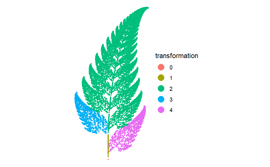
# ℹ 19,991 more rows

Code

ggplot(fern_dat, aes(x, y)) +
  geom_point(colour = "darkgreen", size = 1, stroke = 0) +
  coord_equal() +
  theme_void()

The inclusion of the ‘transform’ column was undertaken purposefully to synchronize with the color aesthetic in the plot. The ensuing visualization delineates discernible patterns: one transformation function dictates the characteristics of the left leaf shape, another prescribes those of the right leaf, and a third shapes the stem. Furthermore, a fourth function systematically duplicates, shifts upward, and rotates its input, yielding the observed vertical symmetry in the output. This deliberate attention to the distinct transformation functions not only enriches the visual representation but also offers insights into the nuanced structural elements portrayed in the plot.

Code

ggplot(fern_dat, aes(x, y, colour = factor(transform))) +
  geom_point(size = 1, stroke = 0) +
  coord_equal() +
  theme_void() + 
  theme(
    legend.text = element_text(colour = "black"),
    legend.title = element_text(colour = "black")
  ) +
  guides(colour = guide_legend(
    title = "transformation", 
    override.aes = list(size = 5))
  )

The lucid manifestation of the impact of each transformation function is now unmistakable. Subsequently, as will be demonstrated shortly, adopting such visualizations proves immensely advantageous. Even when contemplating more intricate color schemes in subsequent stages, the initial depiction of associations between specific functions and their corresponding contributions to the output serves as a valuable diagnostic tool. In my experience, understanding iterated function systems purely through code examination is challenging, given the inherent opacity in the relationship between the code and its output. Consequently, reliance on diagnostic tools, such as visual mappings to iteration numbers, becomes imperative. Without any explicit rationale, the provided fern showcases a color aesthetic mapped to the iteration number, further enhancing interpretability.

Code

ggplot(fern_dat, aes(x, y, colour = iteration)) +
  geom_point(size = 1, stroke = 0, show.legend = FALSE) +
  coord_equal() +
  theme_void()

Code

#------------ Generate the Barnsely Fern ---------------

# Define the coefficients to calculate the x,y values

coef_names <- list(NULL,c("x","y","z"))

coef_x <- matrix(ncol = 3, byrow= TRUE, dimnames = coef_names,
                 c(0, 0, 0,
                   -0.15, 0.28, 0,
                   0.2, -0.26, 0,
                   0.85, 0.04, 0))

coef_y <- matrix(ncol = 3, byrow= TRUE, dimnames = coef_names,
                 c(0, 0.16, 0,
                   0.26, 0.24, 0.44,
                   0.23, 0.22, 1.6,
                   -0.04, 0.85, 1.6))

# Indicate the percentage of iterations through each row of the coefficients
coef_ctrl <- c(1,7,14,85)

# initialize a list to collect the generated points
points <- list()
points$x <- 0
points$y <- 0

# Set maximum iterations and reset coefficient tracker
max_i<-1000000
coef <- NA

# Generate the x,y points as a list and combine as a dataframe
for (i in 2:(max_i)) {
  rand = runif(1, 0, 100)
  
  if (rand < coef_ctrl[1]){coef <- 1} 
  else if (rand < coef_ctrl[2]){coef <- 2}
  else if (rand < coef_ctrl[3]){coef <- 3}
  else {coef <- 4}
  
  points$x[i] <- points$x[i-1]*coef_x[coef, 1] + points$y[i-1]*coef_x[coef, 2] + coef_x[coef, 3]
  points$y[i] <- points$x[i-1]*coef_y[coef, 1] + points$y[i-1]*coef_y[coef, 2] + coef_y[coef, 3]
}
library(dplyr)
df <- bind_rows(points)
# Checkout your Summer Barnsley Fern
plot(df$x, df$y, pch = '.', col = "forestgreen", xaxt = "n", yaxt = "n", xlab = NA, ylab = NA,
     main= "Summer Barnsley Fern")


df$ybin <- signif(df$y,2)

df <- df[-1,] %>% 
  group_by(ybin) %>% 
  mutate(sd = sd(x), mean = mean(x))  %>% 
  ungroup() %>% 
  mutate(xdev = abs(mean -x)/sd)

df[is.na(df$xdev),]$xdev <- 0

# Set the breakpoints and the colors
color_table <- tibble( value = c(0.5, 0.8, 1.1, 1.5, 1.9, 2.1, 2.3, max(df$xdev + (df$y/10))),
                       color = c("forestgreen", "yellowgreen", "yellow3", "gold2",
                                 "darkgoldenrod2", "darkorange3", "darkorange4", "brown4"))

# Lookup the corresponding color for each of the points.
df$col <- NA

for (r in 1:nrow(color_table) ){
  df$col[df$xdev + (df$y/10) <= color_table$value[r] & is.na(df$col)] <- color_table$color[r]
}


plot(df$x, df$y, pch = '.', col = df$col,xaxt = "n", yaxt = "n", xlab = NA, ylab = NA,
     main = "Autumn Barnsley Fern")

4 Brief About Fractal Flame Algorithm

Iterated function systems can be a lot more elaborate than the Barnsley fern, often involving transformation functions that are constructed according to some fancypants compositional rules. For example, the fractal flame algorithm proposed by Scott Draves in 1992 (here’s the original article) specifies transformation functions $f_i()$ – called “flame functions” – that are composed according to the rule:

\[ f_i(\textbf{x}) = \sum_j w_{ij} g_j(\textbf{A}_i \textbf{x}) \]

$\textbf{A}_i$ is a matrix that defines an affine transformation of the coordinates $\textbf{x}$ associated with this specific flame function (i.e., each flame function $f_i()$ has its own transformation , and in the two dimensional case $\textbf{x}$ is just the points $(x,y)$ );
The various $g_j()$ functions are called “variant functions”, and these don’t have to be linear: they can be sinusoidal, or discontinuous, or whatever you like really;
Each flame function is defined as a linear combination of the variant functions: the coefficient $w_{ij}$ specifies the weight assigned to the $j^{\ \text{th}}$ variant function by the $i^{\ \text{th}}$ flame function.

Moreover, analogous to the observations made in the context of the Barnsley fern, it is noteworthy that the flame functions can undergo a nuanced refinement through the incorporation of a probability vector. This introduces a sophisticated layer to the system, allowing for the definition of a bias towards certain flame functions over others.

In this nuanced extension, the algorithm can be imbued with a probabilistic framework, wherein each flame function is assigned a weight based on a probability distribution. Consequently, during the generation process, certain flame functions are more likely to be invoked, introducing a deliberate emphasis on specific visual characteristics. This introduces a level of control and finesse to the output, enabling the artist or programmer to steer the algorithm towards the realization of desired aesthetic nuances within the generated visualizations.

Moreover, akin to the observations elucidated in the context of the Barnsley fern, it is noteworthy that the flame functions, denoted as $f_i(x)$, can undergo a nuanced refinement through the incorporation of a probability vector $\textbf{P}$. This introduces a sophisticated layer to the system, allowing for the definition of a bias towards certain flame functions over others. In this refined model, the algorithm can be imbued with a probabilistic framework, wherein each flame function is assigned a weight based on a probability distribution: $\textbf{P}=(p_1,p_2,…,p_n)$, where $p_i$ represents the probability associated with the $i^{\ \text{th}}$ flame function. Consequently, during the generation process, the invocation of each flame function follows a probabilistic distribution, emphasizing certain functions over others. This deliberate modulation introduces a level of control and finesse to the output, empowering the artist or programmer to steer the algorithm towards the realization of desired aesthetic nuances within the generated visualizations.

In the initial stages of foray into the implementation of the fractal flame algorithm, a deliberate choice was made to eschew the integration of nuanced weighting variables denoted by $w_{ij}$. These elements were purposefully neglected. Subsequently, due to a confluence of fatigue and a lapse in meticulous attention to the subscripts embedded within Draves’ equations, a determination was reached to construct a system wherein each unique combination of a transformation matrix $\textbf{A}_i$ and a variant function $g_j()$ would be accommodated by an individual flame function. The outcome of this deliberation materialized in the form of the ensuing code. Given a set of variant functions $g_1, g_2, \ldots, g_n$, and an ensemble of transformation matrices $\textbf{A}_1,\textbf{A}_2, \ldots,\textbf{A}_m$, the implementation involved the inclusion of every transformation function $f_{ij}(\textbf{x})$ according to the stipulated format:

\[ f_{ij}(\textbf{x}) = g_i(\textbf{A}_i\textbf{x}) \]

In orchestrating these transformation functions in the described fashion, the act of sampling a random transformation, denoted as $f_{ij}$, is facilitated by an independent sampling procedure applied to its dual components. This involves the sequential sampling of a transformation matrix $\textbf{A}_i$ and a variant function $g_j$. The process culminates at this juncture. This distinctive approach represents a peculiar yet intriguing variant within the broader context of the fractal flame algorithm. Despite its departure from conventional methodologies, it unfolds as a nuanced pathway that yields aesthetically pleasing outcomes. This unique interplay of independently sampled transformation elements, involving both matrix and function, contributes to the algorithm’s versatility, showcasing its capacity to produce visually compelling and intricate visualizations.

Now, we will see some computer generated fractal frame art where the coefficients that define the affine transformations $\textbf{A}_i$ have been sampled uniformly at random, with values ranging from $-1$ to $1$.

Code

unboxer_base <- function(iterations, layers, seed = NULL) {
  
  if(!is.null(seed)) set.seed(seed)
  
  # coefficients defining affine layer transforms, A_i
  coeffs <- array(
    data = runif(9 * layers, min = -1, max = 1), 
    dim = c(3, 3, layers)
  )
  
  # list of variant functions, g_j
  funs <- list(
    function(point) point + (sum(point ^ 2)) ^ (1/3),
    function(point) sin(point),
    function(point) 2 * sin(point)
  )
  
  # updater function: apply the layer, then the function
  # (the weirdness with point[3] is me treating colour as special)
  update <- function(point, layer, transform) {
    f <- funs[[transform]]
    z <- point[3]
    point[3] <- 1
    point <- f(point %*% coeffs[,,layer])
    point[3] <- (point[3] + z)/2
    return(point)
  }
  
  # initial point
  point0 <- matrix(
    data = runif(3, min = -1, max = 1), 
    nrow = 1,
    ncol = 3
  )
  
  # sample points
  layer_ind <- sample(layers, iterations, replace = TRUE)  
  trans_ind <- sample(length(funs), iterations, replace = TRUE)  
  points <- accumulate2(layer_ind, trans_ind, update, .init = point0)
  
  # tidy up, add columns, and return
  points <- matrix(unlist(points), ncol = 3, byrow = TRUE)
  points <- cbind(
    points,
    c(0, layer_ind),
    c(0, trans_ind)
  )
  return(points)
}

There are three variant functions $g_j$ in this system: two of them are sinusoidal functions: one of them computes $\sin(x)$ and $\sin(y)$, and the other computes the same thing but multiplies the output by two. Both of these will produce wavy shapes. The other one is a re-scaling function: it tends to shift points towards the top right corner.

At this juncture, it becomes crucial to introduce and underscore the integration of computer-generated values into the current discourse. This introduces a nuanced layer of complexity and sophistication, signifying a pivotal addition that warrants comprehensive elucidation. In essence, these computer-generated values, integral to the ongoing discussion, play a pivotal role in shaping the trajectory of our inquiry. Their introduction broadens the scope of our exploration, infusing a sophisticated computational dimension that merits detailed consideration. These values, emanating from the computational domain, serve as essential elements that contribute to the intricacies of our analysis. Their incorporation into the narrative not only expands the conceptual framework but also establishes a foundation for subsequent discussions on the interplay between theoretical constructs and computational outcomes.

Code

unboxer_base(10, layers = 5, seed = 333)

The first column is the x-coordinate and the second column is the y-coordinate. The third column is a “z-coordinate” that we’ll map to the colour aesthetic later. Column four specifies the layer number (i.e., the value $i$ specifying which affine matrix $\textbf{A}_i$ was used), and column five specifies the variant function number (i.e., the value $j$ specifying which variant function $g_j$ was used).

To transform these numerical values into a visually appealing representation with associated colors, the implementation of a palette function becomes necessary.

Code

sample_canva2 <- function(seed = NULL, n = 4) {
  
  if(!is.null(seed)) set.seed(seed)
  sample(ggthemes::canva_palettes, 1)[[1]] |>
    (\(x) colorRampPalette(x)(n))()  
}

After completing the aforementioned steps, the rendering function, albeit straightforward, serves its purpose effectively. It comprises basic ggplot2 code to generate a scatter plot from the points, with coloration applied using a Canva palette:

Code

unbox_art <- function(data, seed = NULL, size = 1) {
  
  # convert to data frame and sample a palette
  data <- data |> as.data.frame() |> as_tibble()
  names(data) <- c("x", "y", "c", "l", "t")[1:ncol(data)]
  shades <- sample_canva2(seed)
  
  # render image as a scatter plot
  ggplot(data, aes(x, y, colour = c)) +
    geom_point(
      size = size,
      stroke = 0,
      show.legend = FALSE
    ) + 
    theme_void() + 
    coord_equal(xlim = c(-4, 4), ylim = c(-4, 4)) + 
    scale_colour_gradientn(colours = shades) + 
    scale_x_continuous(expand = c(0, 0)) +
    scale_y_continuous(expand = c(0, 0)) +
    theme(panel.background = element_rect(
      fill = shades[1], colour = shades[1]
    ))
}

Indeed, the aesthetic appeal is notably enhanced when a substantial number of points, such as 3 million, are generated and plotted with a diminutive marker size, e.g., 0.1. This approach not only accentuates the intricacies of the rendered fern but also contributes to a visually striking and finely detailed representation. The combination of a large dataset and a small marker size serves to amplify the artistic quality and overall visual impact of the generated plot.

Code

mil <- 1000000
tic()
unboxer_base(3 * mil, layers = 3, seed = 66) |> 
  unbox_art(seed = 66, size = .1)

The computational efficiency of the system is moderate. Nevertheless, we will discuss shortly the implementation of measures to notably expedite this process.

Code

tic()
unboxer_base(mil, layers = 2, seed = 999) |> unbox_art(seed = 2, size = .2)
unboxer_base(mil, layers = 5, seed = 333) |> unbox_art(seed = 2, size = .2) 
unboxer_base(mil, layers = 9, seed = 420) |> unbox_art(seed = 2, size = .2)
toc()

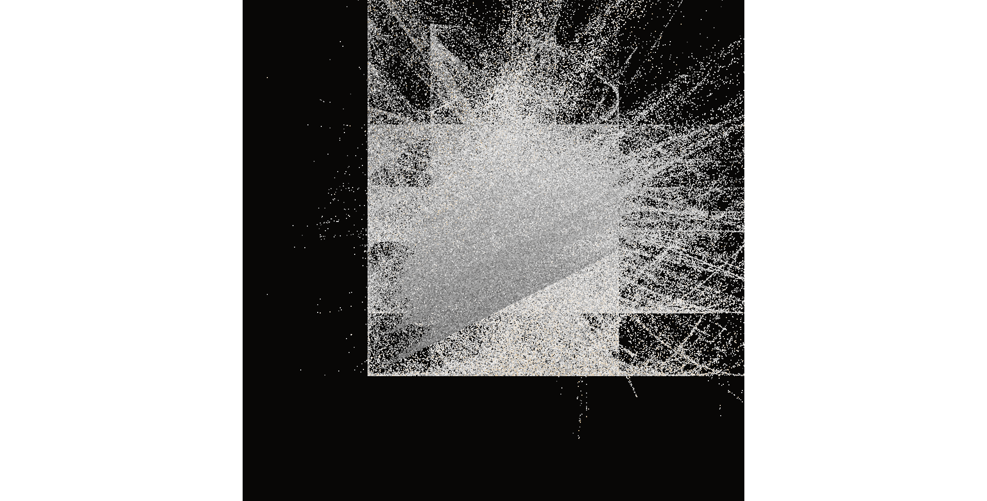
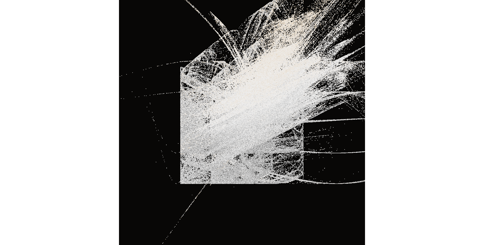
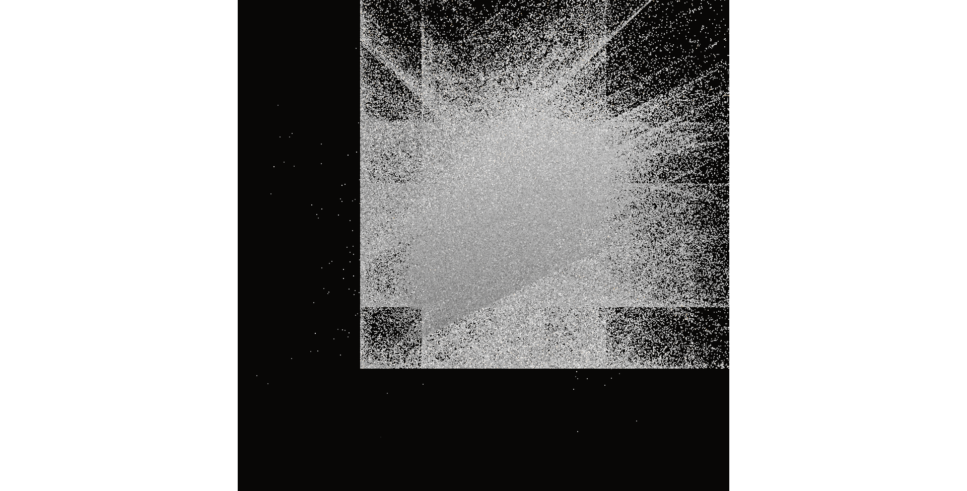
The outputs from this system exhibit a consistent visual motif: a pair of nested boxes with an emergent element emanating from the top-right corner. While the broad structure remains uniform, the finer details exhibit substantial variation across different outputs. Notably, there are discernible systematic differences contingent on the number of layers employed. The provided example illustrates the impact on the output as the number of layers progresses incrementally from 2 to 9, revealing a nuanced evolution in the complexity and intricacy of the generated patterns.

To comprehend the dynamics of this system, we will undertake a similar approach as we did with the Barnsley fern. we will generate the data for an artwork by invoking unboxer_base(), followed by three distinct visualizations. Initially, we will present a pure black and white image to elucidate the overall arrangement of points. Subsequently, we will deconstruct it based on the components. Given that each transformation function is delineated in terms of the affine and variant components, we will provide two distinct versions to elucidate these aspects.

Code

dat <- unboxer_base(mil, layers = 2, seed = 99) |> 
  as.data.frame() |> 
  as_tibble()

names(dat) <- c("x", "y", "c", "affine_layer", "variant_function")

dat <- dat |> 
  slice_tail(n = -1) |> 
  mutate(
    affine_layer = factor(affine_layer),
    variant_function = factor(variant_function)
  ) 

ggplot(dat, aes(x, y)) +
  geom_point(size = .4, stroke = 0, show.legend = FALSE) + 
  theme_void() + 
  coord_equal(xlim = c(-4, 4), ylim = c(-4, 4))
ggplot(dat, aes(x, y, colour = variant_function)) +
  geom_point(size = .4, stroke = 0) + 
  coord_equal(xlim = c(-4, 4), ylim = c(-4, 4)) +
  scale_colour_brewer(palette = "Set2") +
  guides(colour = guide_legend(nrow = 1, override.aes = list(size = 5))) +
  theme_void() + 
  theme(legend.position = c(0.2, 0.1))
ggplot(dat, aes(x, y, colour = affine_layer)) +
  geom_point(size = .4, stroke = 0) + 
  coord_equal(xlim = c(-4, 4), ylim = c(-4, 4)) +
  scale_colour_brewer(palette = "Set1") +
  guides(colour = guide_legend(nrow = 1, override.aes = list(size = 5))) +
  theme_void() + 
  theme(legend.position = c(0.2, 0.1))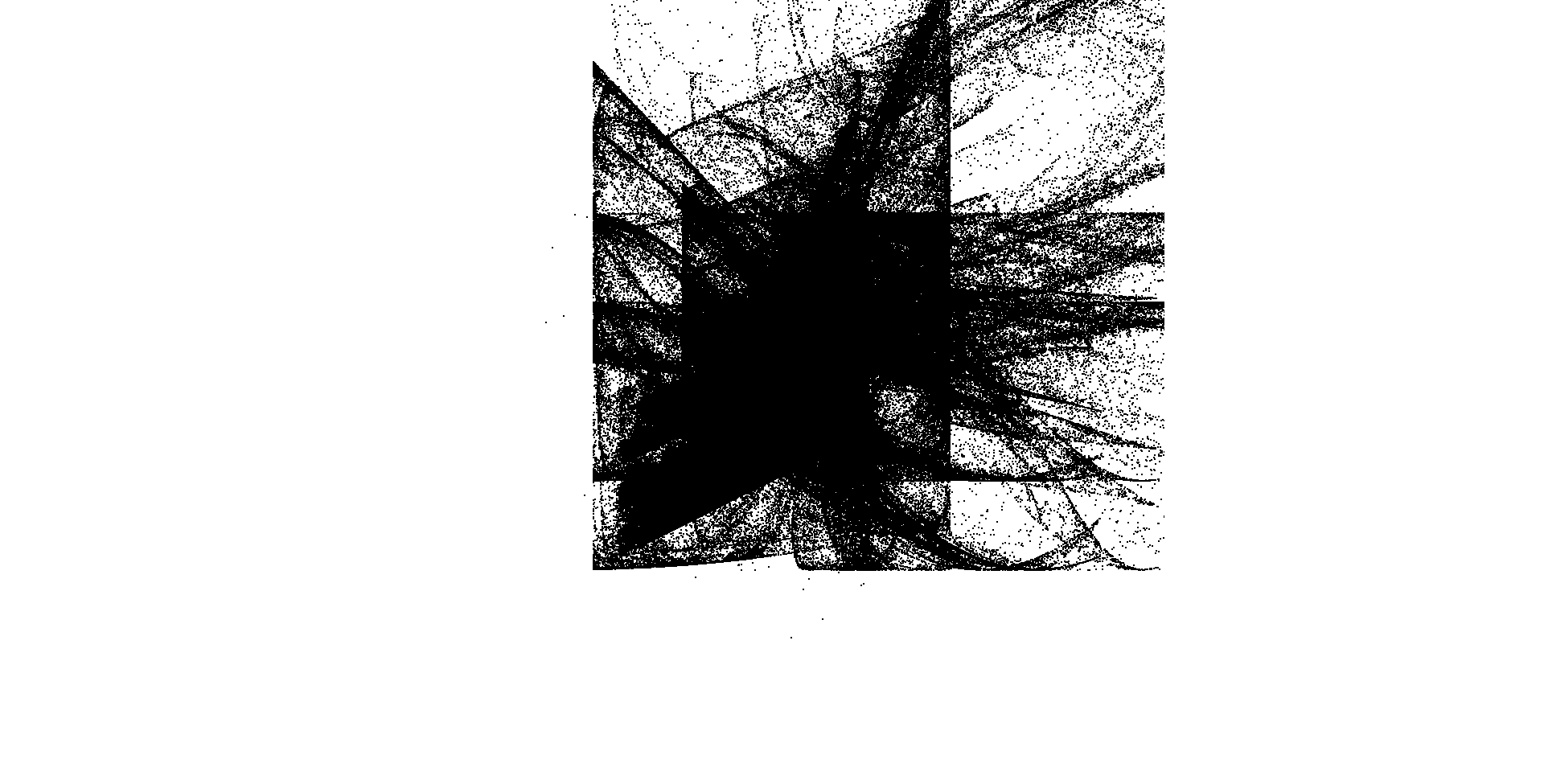

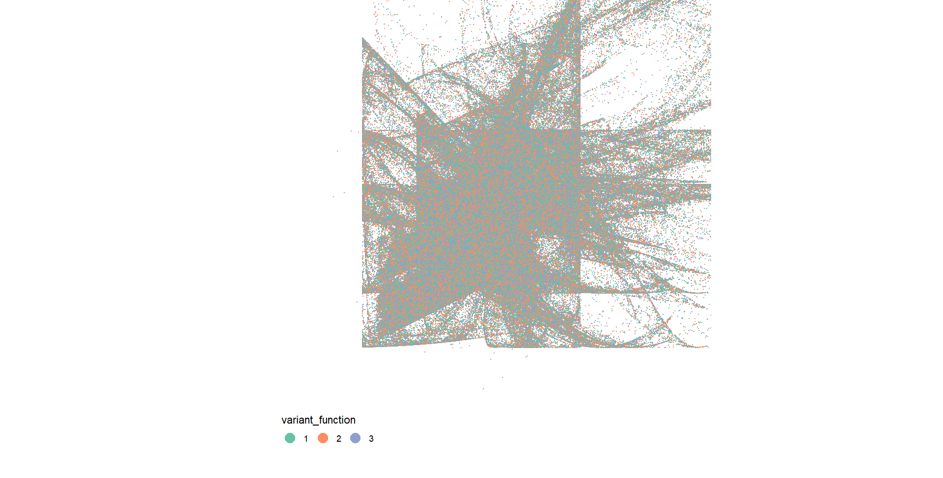
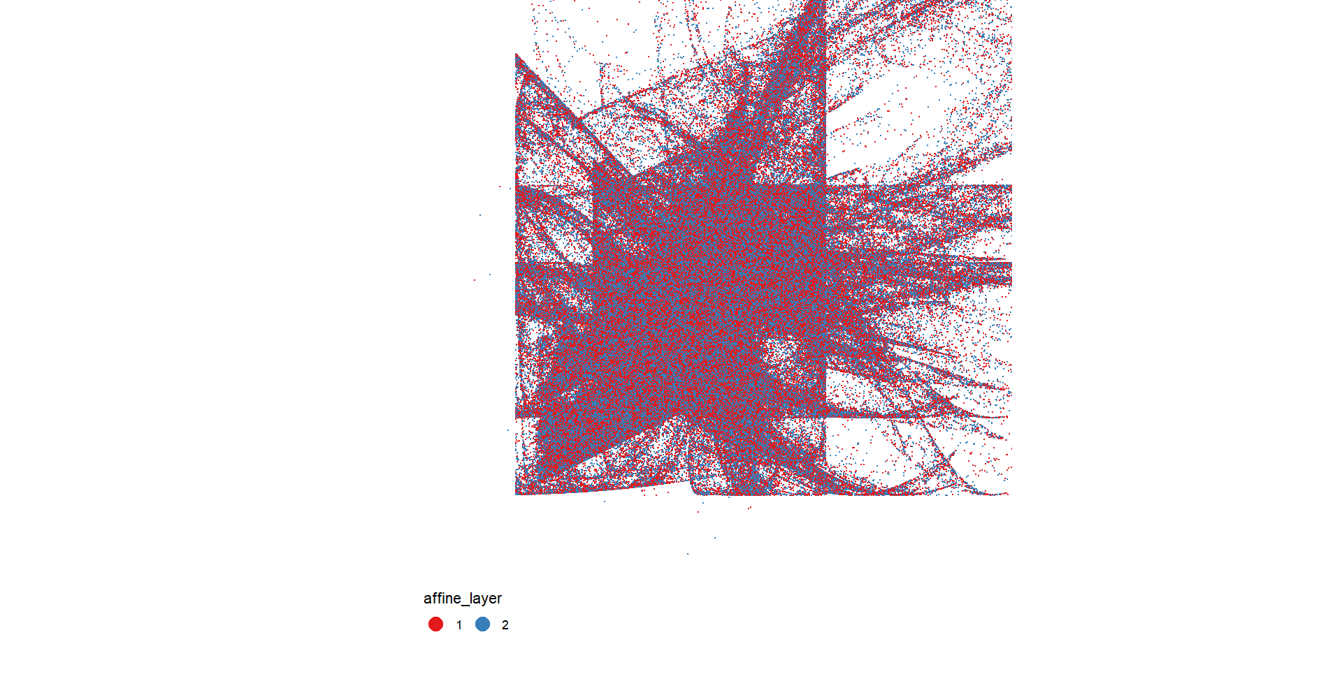
This comprehensive analysis affords a profound understanding of the intricate processes at play within the depicted visuals. Focusing on the central panel, the observable manifestation of geometric patterns is inherently tied to the influence exerted by the two distinct “sinusoidal” components. The key to this phenomenon lies in the inherent constraints of the sine function, which, confined within the range of -1 to 1, gives rise to the formation of discernible boxes. However, it is imperative to note that the intricate, undulating patterns apparent in select outputs bear an inherent relationship with these sinusoidal components, although the graphical representation may not overtly elucidate this nuanced association.

In deliberate contrast, the panel situated on the right of the visual display unveils a lucid portrayal of the transformative impact arising from the application of affine transformations. It is particularly noteworthy that the blue pattern assumes a semblance to a “squashed and rotated” rendition of the red pattern. This observation encapsulates the precise function of affine transforms – introducing deliberate distortions that imbue the generated outputs with a distinctive visual character. This nuanced exploration not only enhances our appreciation of the graphical representations but also serves as a foundation for delving deeper into the intricate interplay of mathematical constructs and visual outcomes.

Conclusion

In conclusion, the multifaceted exploration of geometric patterns and visual outcomes, as elucidated through the interplay of sinusoidal components and affine transformations, opens avenues for further research and investigation. This preliminary analysis provides a foundational understanding of the underlying dynamics, shedding light on the constraints imposed by mathematical functions and the transformative potential inherent in affine operations. To propel this inquiry forward, a promising avenue for future research involves a more granular examination of the nuanced relationships between specific mathematical components and their visual manifestations. Exploring the potential variations in constraints, modifying parameters, or introducing additional elements could unearth deeper insights into the rich tapestry of geometric patterns generated through computational processes.

Furthermore, an in-depth exploration of the role of probability vectors, as mentioned earlier, could serve as a catalyst for advancing the sophistication of these generative algorithms. Investigating the impact of weighted probabilities on the prevalence of certain visual features could contribute to the refinement of aesthetic control in the output. Additionally, considering the broader implications of these generative processes, both from an artistic and mathematical standpoint, opens up interdisciplinary avenues. Collaborations between mathematicians, artists, and computer scientists could foster innovative approaches, leading to the creation of visually compelling outputs that not only adhere to mathematical principles but also push the boundaries of artistic expression.

In essence, the presented analysis lays the groundwork for a more intricate exploration of generative algorithms, paving the way for future investigations that delve deeper into the mathematical intricacies and artistic potential inherent in these computational systems. The journey towards unraveling the full extent of these generative capabilities promises to be both challenging and rewarding, offering rich opportunities for interdisciplinary collaboration and creative exploration.

Footnotes

References

Fractals Everywhere, Boston, MA: Academic Press, 1993, ISBN 0-12-079062-9
https://flam3.com/flame_draves.pdf
Falconer, Kenneth (1990). Fractal geometry: Mathematical foundations and applications. John Wiley and Sons. pp. 113–117, 136. ISBN 0-471-92287-0.
Barnsley, Michael; Andrew Vince (2011). “The Chaos Game on a General Iterated Function System”. Ergodic Theory Dynam. Systems. 31 (4): 1073–1079. arXiv:1005.0322. Bibcode:2010arXiv1005.0322B. doi:10.1017/S0143385710000428. S2CID 122674315.
Draves, Scott; Erik Reckase (July 2007). “The Fractal Flame Algorithm” (PDF). Archived from the original (PDF) on 2008-05-09. Retrieved 2008-07-17.
Dietmar Saupe, Raouf Hamzaoui. “A Review of the Fractal Image Compression Literature”
Bauschke, Heinz H. (2017). Convex Analysis and Monotone Operator Theory in Hilbert Spaces. New York: Springer.

--- title: "Analyzing Fractal Complexity" subtitle: "A Comprehensive Examination of Iterated Function Systems in Mathematical and Computational Sciences" author: "Abhirup Moitra" date: 2023-12-10 format: html: code-fold: true code-tools: true editor: visual categories : [Mathematics, R Programming] image: fern-asimg.jpg --- ![](fractal-pattern.jpg){fig-align="center" width="328"} ::: {style="color: navy; font-size: 20px; font-family: Garamond; text-align: center; border-radius: 3px; background-image: linear-gradient(#C3E5E5, #F6F7FC);"} **Nature builds up her refined and invisible architecture with a delicacy eluding our conception** ::: # **Abstract** This research project delves into the domain of **Iterated Function Systems (IFS),** a mathematical framework within fractal geometry renowned for its capacity to produce intricate self-replicating patterns. The inquiry begins with an elucidation of the core components constituting an IFS, which involves a set of contraction mappings defined by mathematical functions. These functions, recognized for their contractive nature, iteratively transform points within a given space. Integral to the methodology of **IFS** is the integration of probabilities associated with each transformation, influencing the likelihood of selecting a specific function during the iterative process. Through the repetitive application of these functions and the infusion of randomness via probability weights, a sequence of points evolves, converging towards a fractal structure identified as the limit set. The study scrutinizes the convergence characteristics of IFS and the manifestation of self-similar patterns within the limit set. By examining the interplay between simplicity at the function level and the observed complexity at the macroscopic fractal level, the research underscores the captivating nature of **IFS** in generating visually compelling and intricate structures. Practical applications of **IFS** are explored, ranging from its role in computer graphics to applications in image compression techniques. The abstract nature of fractal patterns generated by **IFS** finds utility in diverse fields, offering a versatile tool for creating realistic, natural forms with self-repeating characteristics. In conclusion, this exploration of Iterated Function Systems contributes to a deeper understanding of the mathematical principles underpinning fractal geometry and its applications in computer science. The study aims to underscore the significance of IFS as a powerful and flexible tool for generating complex, self-replicating structures with applications that extend across various domains of scientific inquiry and artistic expression. # **1. Basic Formalism** ## **1.1 Metric Space** A metric space is a mathematical structure that formalizes the concept of distance between points. It is a set equipped with a distance function (metric) that satisfies certain properties. The distance function assigns a non-negative real number to pairs of points in the set, representing the distance between those points. ## **Definition** A **metric space** consists of a set X and a metric $d: X \times X \to \mathbb{R}$ such that for any points $x,y,z$ in $X$, the following conditions, called the metric axioms, are satisfied: 1. **Non-negativity:** $d(x,y) \ge 0$ (distance is always non-negative). 2. **Identity of indiscernibles:** $d(x,y)=0$ if and only if $x=y$ (distinct points have positive distance). 3. **Symmetry:** $d(x,y)=d(y,x)$ (the distance between two points is the same regardless of the order). 4. **Triangle inequality:** $d(x,y)+d(y,z)≥d(x,z)$ (the direct route is always at least as short as any detour). ![](Manhattan_distance.jpg){fig-align="center" width="226"} The [plane](#0 "Two-dimensional Euclidean space") (a set of points) can be equipped with different metrics. In the [taxicab metric](#0 "Taxicab geometry") the red, yellow, and blue paths have the same [length](#0 "Arc length") (12), and are all the shortest paths. In the Euclidean metric, the green path has length $6 \sqrt{2} \approx 8.49$, and is the unique shortest path, whereas the red, yellow, and blue paths still have a length of $12$. ## **1.2 Cauchy Sequence** A **Cauchy sequence** is a [sequence](#0 "Sequence") whose [elements](#0 "Element (mathematics)") become arbitrarily close to each other as the sequence progresses. More precisely, given any small positive distance, all excluding a finite number of elements of the sequence are less than that given distance from each other. ## **Definition** $\text{Let}\; (X,d)\; \text{be a metric space. Then}\; \{x_n\}_{n\ge1} \subseteq X\; \text{is called a Cauchy sequence if}\;$ $$ \forall \epsilon >0\ \exists N\in \mathbb{N}\ \forall m,n \ge N\;\;\ d(x_m,x_n) < \epsilon $$ ## **1.3 Complete Metric Space** A metric space $(X,d)$ is called complete if every Cauchy sequence in that space converges to a limit that is also within the space. ::: {style="font-family: Georgia; text-align: center; font-size: 19px"} ***This means that there are no "missing" points, and the space is closed under the limit operation for Cauchy sequences.*** ::: ## **1.2 Iterated function** Let $X$ be a set and $f: X \to X$ be a [function](#0 "Function (mathematics)"). Defining $f^n$ as the $n^\text{th}$ iterate of $f$. where $n$ is a non-negative integer. An **iterated function** is a function $X \to X$ (that is, a function from some [set](#0 "Set (mathematics)") $X$ to itself) which is obtained by [composing](#0 "Function composition") another function $f : X \to X$ with itself a certain number of times. The process of repeatedly applying the same function is called [iteration](#0 "Iteration"). In this process, starting from some initial object, the result of applying a given function is fed again into the function as input, and this process is repeated. $$ L = F(k) , M = F \circ F (k) = F^2(k) $$ For example on the image on the bottom ![](An_iterated_direct_similarity_yields_spirals.jpg){fig-align="center" width="300"} ## **1.3 Iterated Function System(IFS)** Formally, an **iterated function system(IFS)** is a finite set of [contraction mappings](#0 "Contraction mapping") on a [complete metric space](#0 "Complete metric space"). Symbolically, $$ \{f_i : X \to X\ | \ i = 1,2,\ldots N\} \;\text{where}\; N \in \mathbb{N} $$ is an iterated function system if each $f_i$ is a contraction on the complete metric space $X$. Hutchinson showed that, for the metric space $\mathbb{R}^n$, or more generally, for a complete metric space $X$, such a system of functions has a unique nonempty [compact](https://en.wikipedia.org/wiki/Compact_space "Compact space") (closed and bounded) fixed set *S*.^[\[3\]](https://en.wikipedia.org/wiki/Iterated_function_system#cite_note-hutchinson-3)^ One way of constructing a fixed set is to start with an initial nonempty closed and bounded set *S*~0~ and iterate the actions of the $fi$, taking $S_{n+1}$to to be the union of the images of $S_n$ under the $fi$; then taking $S$ to be the [closure](#0 "Closure (topology)") of the limit $\displaystyle\lim_{n \to \infty} S_n$. Symbolically, the unique fixed (nonempty compact) set $S \subseteq X$ has the property. $$ S = \overline{\bigcup_{i=1}^N f_i(S)} $$ The set $S$ is thus the fixed set of the Hutchinson operator $F: 2^X \to 2^X$ defined $A \subseteq X$ via $$F(A) =\overline{\bigcup_{i=1}^N f_i(A)} $$ The existence and uniqueness of $S$ is a consequence of the contraction mapping principle, as is the fact that $$ \lim_{n \to \infty} F^n(A) = S $$ for any nonempty compact set $A$ in $X$. (For contractive IFS this convergence takes place even for any nonempty closed bounded set $A$). Random elements arbitrarily close to $S$may be obtained by the "**chaos game**," # 2. Contraction Mapping An IFS involves a finite collection of functions. Each function in the set represents a transformation. Contractive maps, also known as contractions, are functions that bring points closer together. Specifically, a function $f$ is contractive if there exists a constant $0 \le k<1$ such that for any two points $x$ and $y$, the distance between $f(x)$ and $f(y)$ is less than $k$ times the distance between $x$ and $y$. ## **Definition** A **contraction mapping**, or **contraction** on a [metric space](#0 "Metric space") $(M, d)$ is a [function](#0 "Function (mathematics)") $f$ from $M$ to itself, with the property that there is some [real number](#0 "Real number") $0 \le k<1$ such that $\forall x,y \in M.$ $$ d(f(x), f(y)) \le k.d(x,y) $$ The smallest such value of $k$ is called the **Lipschitz constant** of $f$. Contractive maps are sometimes called **Lipschitzian maps**. If the above condition is instead satisfied for $k\le 1$, then the mapping is said to be a [non-expansive map](https://en.wikipedia.org/wiki/Non-expansive_map "Non-expansive map"). More generally, the idea of a contractive mapping can be defined for maps between metric spaces. Thus, if $(M, d)$ and $(N, d')$ are two metric spaces, then $f : M \to N$ is a contractive mapping if there is a constant $0 \le k<1$ such that, $$ d'(f(x), f(y)) \le k.d(x,y)\; \forall x,y \in M $$ Complete Metric Space,the functions in an **IFS** operate on a complete metric space. A metric space is a set equipped with a distance function (metric) that satisfies certain properties. Completeness implies that every Cauchy sequence in the space converges to a limit that is also within the space. The process of an Iterated Function System involves repeatedly applying these contractive maps to points in the metric space. This iteration can lead to interesting and complex patterns. IFS is commonly used in the field of fractal geometry to generate self-replicating structures and patterns. One well-known example of an IFS is the construction of the Sierpinski triangle. Each function in the IFS is a contraction that transforms an equilateral triangle into a smaller equilateral triangle. Through iteration, this process generates the intricate **Sierpinski triangle** pattern. # 3 Chaotic Realm We have already come across the definition of an **Iterated Function System(IFS)** where each $f_i$ is a contraction on the complete metric space $X$. Each function $f_i$ is required to be a linear, or more generally an [affine](https://en.wikipedia.org/wiki/Affine_transformation "Affine transformation"), transformation, and hence represented by a matrix. However, IFSs may also be built from non-linear functions, including [projective transformations](https://en.wikipedia.org/wiki/Projective_transformation "Projective transformation") and [Möbius transformations](https://en.wikipedia.org/wiki/M%C3%B6bius_transformation "Möbius transformation"). The [Fractal flame](https://en.wikipedia.org/wiki/Fractal_flame "Fractal flame") is an example of an IFS with nonlinear functions. The most common algorithm to compute IFS fractals is called the "[chaos game](https://en.wikipedia.org/wiki/Chaos_game "Chaos game")". It consists of picking a random point in the plane, and then iteratively applying one of the functions chosen at random from the function system to transform the point to get a next point. An alternative algorithm is to generate each possible sequence of functions up to a given maximum length, and then plot the results of applying each of these sequences of functions to an initial point or shape. Each of these algorithms provides a global construction that generates points distributed across the whole fractal. If a small area of the fractal is being drawn, many of these points will fall outside of the screen boundaries. This makes zooming into an IFS construction drawn in this manner impractical. Although the theory of IFS requires each function to be contractive, in practice software that implements IFS only requires that the whole system be contractive on average. ## **3.1 Chaos Game** The chaos game is an engaging and intuitive way to explore the fractal structures generated by IFS transformations. By iteratively applying random transformations to points in a space, you can observe the emergence of intricate and self-replicating patterns. In a research or coding project focused on IFS, incorporating the chaos game serves both educational and practical purposes. Here are some points you might consider emphasizing or exploring further. ## **3.2 Chaos Game For The Barnsley Fern** The fern is one of the basic examples of self-similar sets, i.e. it is a mathematically generated pattern that can be reproducible at any magnification or reduction. Barnsley's 1988 book *Fractals Everywhere* is based on the course that he taught for undergraduate and graduate students in the School of Mathematics, **Georgia Institute of Technology**, called *Fractal Geometry*. After publishing the book, a second course was developed, called *Fractal Measure Theory*. Barnsley's work has been a source of inspiration to graphic artists attempting to imitate nature with mathematical models. The fern code developed by Barnsley is an example of an iterated function system (IFS) to create a fractal. This follows from the *collage theorem*. He has used fractals to model a diverse range of phenomena in science and technology, but most specifically plant structures. ### **3.2.1 Collage Theorem** the **collage theorem** characterizes an iterated function system whose attractor is close, relative to the [Hausdorff metric](#0 "Hausdorff metric"), to a given set. The IFS described is composed of contractions whose images, as a **collage** or union when mapping the given set, are arbitrarily close to the given set. It is typically used in [fractal compression](#0 "Fractal compression"). #### **Statement** Let $\mathbb{X}$ be a *complete metric space*. Suppose $L$ is a nonempty, *compact subset* of $\mathbb{X}$ and let $\epsilon >0$ be given. Choose an iterated function system (IFS) $\{\mathbb{X};\ w_1, w_2, \ldots w_N\}$ with contractivity factor $s$ where $0 \le s < 1$ (the contractivity factor $s$ of the IFS is the maximum of the contractivity factors of the maps $w_i$). Suppose $$ h\Bigg(L, \bigcup_{n=1}^N w_n(L)\Bigg) \le \epsilon $$ where $h(.,.)$ is the [Hausdorff metric](https://en.wikipedia.org/wiki/Hausdorff_distance "Hausdorff distance"). Then $$ h(L,A) \le \frac{\epsilon}{1-s} $$ where $A$ is the attractor of the IFS. Equivalently, $h(L,A) \le (1-s)^{-1}\ h(L,\cup_{n=1}^N w_n(L))$ for all non-empty subset $L$ of $\mathbb{X}$. **Remark:** Barnsley's fern uses four *affine transformations*. The formula for one transformation is the following: $$ f(x,y) = \begin{bmatrix} \ a \ & \ b & \\ \ c & \ d \end{bmatrix} \begin{bmatrix} x \\ \ y \end{bmatrix} +\begin{bmatrix} e \\ \ f \end{bmatrix} $$ Barnsley shows the *IFS* code for his *Black Spleenwort* fern fractal as a matrix of values shown in a table. In the table, the columns "a" through "f" are the coefficients of the equation and "p" represents the probability factor. So let's introduce what is affine transformation, then we'll introduce the pseudo-code of *Barnsley Fern*. ## **3.2.2 Affine Transformations** An affine transformation is an automorphism of an affine space (Euclidean spaces are specific affine spaces), that is, a function which maps an affine space onto itself while preserving both the dimension of any affine subspaces (meaning that it sends points to points, lines to lines, planes to planes, and so on) and the ratios of the lengths of parallel line segments. Consequently, sets of parallel affine subspaces remain parallel after an affine transformation. An affine transformation does not necessarily preserve angles between lines or distances between points, though it does preserve ratios of distances between points lying on a straight line. If $X$ is the point set of an affine space, then every affine transformation on $X$ can be represented as the composition of a linear transformation on $X$ and a translation of $X$. Unlike a purely linear transformation, an affine transformation need not preserve the origin of the affine space. Thus, every linear transformation is affine, but not every affine transformation is linear. A generalization of an affine transformation is an affine map between two (potentially different) affine spaces over the same field $\mathbb{K}$. Let $(X, V, \mathbb{K})$ and $(Z, W, \mathbb{K})$ be two affine spaces with $X$ and $Z$ the point sets and $V$ and $W$ the respective associated vector spaces over the field $\mathbb{K}$. A map $f: X \to Z$ is an affine map if there exists a linear map $m_f : V \to W$ such that $m_f (x − y) = f (x) − f (y) \forall x, y \in X$. ### **Definition** Let $X$ be an affine space over a field $k$, and $V$ be its associated vector space. An affine transformation is a bijection $f$ from $X$ onto itself that is an affine map; this means that a linear map $g$ from $V$ to $V$ is well defined by the equation $g(y-x) = f(y) - f(x);$ here, as usual, the subtraction of two points denotes the [free vector](https://en.wikipedia.org/wiki/Free_vector "Free vector") from the second point to the first one, and "[well-defined](https://en.wikipedia.org/wiki/Well-defined "Well-defined")" means that $y-x = y'-x'$ implies that $f(y)- f(x) =f(x') - f(y')$ If the dimension of $X$ is at least two, a *semiaffine transformation* $f$ of $X$ is a [bijection](#0 "Bijection") from $X$ onto itself satisfying: 1. For every *d*-dimensional [affine subspace](https://en.wikipedia.org/wiki/Affine_subspace "Affine subspace") $S$ of $X$, then $f (S)$ is also a *d*-dimensional affine subspace of $X.$ 2. If $S$ and $T$ are parallel affine subspaces of $X$, then $f (S)$ and $f (T)$ are parallel. ### Structure By the definition of an affine space, $V$ acts on $X$, so that, for every pair $(x, v)$ in $X × V$ there is associated a point $y$ in $X$. We can denote this action by $\vec{v}(x) = y$. Here we use the convention that $\vec{v} =v$ are two interchangeable notations for an element of $V$. By fixing a point $c$ in $X$ one can define a function $m_c : X → V\; by\; m_c(x) = \vec{cx}$. For any $c$, this function is one-to-one, and so, has an inverse function $m_c^{−1} : V → X$ given by $m_c^{−1}(v) = \vec{v}(c)$. These functions can be used to turn $X$ into a vector space (concerning the point $c$) by defining: - $x+y = m_c^{-1}(m_c(x)+m_c(y)), \forall x,y \in X$ - $rx = m_c^{-1}(rm_c(x)), \forall r \in k\; \& \; x \in X$ This vector space has origin $c$ and formally needs to be distinguished from the affine space $X$, but common practice is to denote it by the same symbol and mention that it is a vector space after an origin has been specified. This identification permits points to be viewed as vectors and vice versa. For any linear transformation $\lambda$ of $V$, we can define the function $L(c, \lambda) : X → X$ by, $$L(c, \lambda)(x) = m_c^{-1}(\lambda (m_c(x))) = c+ \lambda(\overrightarrow{cx})$$Then $L(c, \lambda)$ is an affine transformation of $X$ which leaves the point $c$ fixed. It is a linear transformation of $X$, viewed as a vector space with origin $c$. ### **Affine Maps** Given two affine spaces $\mathcal{A}$ and $\mathcal{B}$, over the same field, a function $f: \mathcal{A \to B}$ is an affine map if and only if for every family $\{(a_i,\lambda_i)\}_{i \in I}$ of weighted points in $\mathcal{A}$ such that, $$ \sum_{i \ \in \ I} \lambda_i = 1 $$ $$ f\bigg(\sum_{i \ \in \ I} \lambda_i \ a_i \bigg) = \sum_{i \ \in \ I} \lambda_if(a_i) $$ An affine map $\mathcal{f: A \to B}$ between two affine spaces is a map on the points that acts linearly on the vectors (that is, the vectors between points of the space). In symbols, $f$ determines a linear transformation $\phi$ such that, for any pair of points $P,Q \in \mathcal{A}$: $$\overrightarrow{f(P) f(Q)} = \phi(\overrightarrow{PQ})$$ or , $$ f(Q) - f(P) = \phi(Q-P) $$ We can interpret this definition in a few other ways, as follows. If an origin $O \in \mathcal{A}$ is chosen , and $B$ denotes its image $f(O) \in \mathcal{B}$ then this means that for any vectors $\vec{x}$: $$f:(O+\vec{x}) \to (B+ \phi(\vec{x}))$$ If an origin $O' \in \mathcal{B}$ is also chosen, this can be decomposed as an affine transformation $g:\mathcal{A \to B}$ that sends $O \to O'$ namely, $$f:(O+\vec{x}) \to (O'+ \phi(\vec{x}))$$ followed by the translation by a vector $\vec{b} = \overrightarrow{O'B}.$ The conclusion is that, intuitively, $f$ consists of a translation and linear map. ## **3.2.3 Generate** Barnsley Fern We have written the assumption that the functions are defined over a two dimensional space with $x$ and $y$ coordinates, but it generalizes naturally to any number of dimensions. When choosing a transformation function in step 3, you can sample uniformly at random, or impose a bias so that some transformation are applied more often than others. To get a sense of how this works, let's start with a classic example: the Barnsley fern. The Barnsley fern, like many iterated function systems used for the art, is constructed from functions $f(x,y)$ defined in two dimensions. Better yet, they're all affine transformations. So we write any such function down using good old fashioned linear algebra, and compute everything using matrix multiplication and addition: $$ f(x,y) = \begin{bmatrix} \ a \ & \ b & \\ \ c & \ d \end{bmatrix} \begin{bmatrix} x \\ \ y \end{bmatrix} +\begin{bmatrix} e \\ \ f \end{bmatrix} $$ Four functions build the Barnsley fern, with the coefficients listed below: | function | $a$ | $b$ | $c$ | $d$ | $e$ | $f$ | $p$ | interpretation | |--------|--------|--------|--------|--------|--------|--------|--------|--------| | $f_1(x,y)$ | 0 | 0 | 0 | 0.16 | 0 | 0 | 0.01 | stem | | $f_2(x,y)$ | 0.85 | 0.04 | -0.04 | 0.85 | 0 | 1.60 | 0.85 | ever-smaller leaflets | | $f_3(x,y)$ | 0.20 | -0.26 | 0.23 | 0.22 | 0 | 1.60 | 0.07 | largest left-hand leaflet | | $f_4(x,y)$ | -0.15 | 0.28 | 0.26 | 0.24 | 0 | 0.44 | 0.07 | largest right-hand leaflet | $$ f_1(x,y) = \begin{bmatrix} \ 0.00 \ & \ 0.00 & \\ \ 0.00 & \ 0.16 \end{bmatrix} \begin{bmatrix} x \\ \ y \end{bmatrix} $$ $$ f_2(x,y) = \begin{bmatrix} \ 0.85 \ & \ 0.04 & \\ -0.04\ & \ 0.85 \end{bmatrix} \begin{bmatrix} x \\ \ y \end{bmatrix} +\begin{bmatrix} 0.00 \\ \ 1.60 \end{bmatrix} $$ $$ f_3(x,y) = \begin{bmatrix} \ 0.20 \ & \ -0.26 & \\ \ 0.23 & \ 0.22 \end{bmatrix} \begin{bmatrix} x \\ \ y \end{bmatrix} +\begin{bmatrix} 0.00 \\ \ 1.60 \end{bmatrix} $$ $$ f_4(x,y) = \begin{bmatrix} \ -0.15 \ & \ 0.28 & \\ \ 0.26 & \ 0.24 \end{bmatrix} \begin{bmatrix} x \\ \ y \end{bmatrix} +\begin{bmatrix} 0.00 \\ \ 0.44 \end{bmatrix} $$ The first point drawn is at the origin $(x_0 = 0, y_0 = 0)$ and then the new points are iteratively computed by randomly applying one of the following four coordinate transformations: *ƒ*~1~ *x~n~* ~+ 1~ = 0 *y~n~* ~+ 1~ = 0.16 *y~n~* This coordinate transformation is chosen 1% of the time and just maps any point to a point in the first line segment at the base of the stem. In the iterative generation, it acts as a reset to the base of the stem. Crucially it does not reset exactly to $(0,0)$ which allows it to fill in the base stem which is translated and serves as a kind of "kernel" from which all other sections of the fern are generated via transformations $ƒ_2, ƒ_3, ƒ_4.$ *ƒ*~2~ *x~n~* ~+ 1~ = 0.85 *x~n~* + 0.04 *y~n~* *y~n~* ~+ 1~ = −0.04 *x~n~* + 0.85 *y~n~* + 1.6 This transformation encodes the self-similarity relationship of the entire fern with the sub-structure which consists of the fern with the removal of the section which includes the bottom two leaves. In the matrix representation, it can be seen to be a slight clockwise rotation, scaled to be slightly smaller and translated in the positive y direction. In the iterative generation, this transformation is applied with probability 85% and is intuitively responsible for the generation of the main stem, and the successive vertical generation of the leaves on either side of the stem from their "original" leaves at the base. *ƒ*~3~ *x~n~* ~+ 1~ = 0.2 *x~n~* − 0.26 *y~n~* *y~n~* ~+ 1~ = 0.23 *x~n~* + 0.22 *y~n~* + 1.6 This transformation encodes the self-similarity of the entire fern with the bottom left leaf. In the matrix representation, it is seen to be a near-90° counter-clockwise rotation, scaled down to approximately 30% size with a translation in the positive y direction. In the iterative generation, it is applied with probability 7% and is intuitively responsible for the generation of the lower-left leaf. *ƒ*~4~ *x~n~* ~+ 1~ = −0.15 *x~n~* + 0.28 *y~n~* *y~n~* ~+ 1~ = 0.26 *x~n~* + 0.24 *y~n~* + 0.44 Similarly, this transformation encodes the self-similarity of the entire fern with the bottom right leaf. From its determinant it is easily seen to include a reflection and can be seen as a similar transformation as *ƒ*~3~ albeit with a reflection about the y-axis. In the iterative-generation, it is applied with probability 7% and is responsible for the generation of the bottom right leaf. ### **Pseudocode** ``` draw all pixels on screen white x = 0.0 y = 0.0 n = 0.0 xn = 0.0 yn = 0.0 while n < maximum iterations: r = random() between 0 and 1 if r < 0.01 xn = 0.0 yn = 0.16 * y else if r < 0.86 xn = 0.85 * x + 0.04 * y yn = -0.04 * x + 0.85 * y + 1.6 else if r < 0.93 xn = 0.2 * x - 0.26 * y yn = 0.23 * x + 0.22 * y + 1.6 else xn = -0.15 * x + 0.28 * y yn = 0.26 * x + 0.24 * y + 0.44 draw pixel (xn, yn) green on screen x = xn y = yn increment n ``` ### **Computer Generation** ```{r, message=FALSE,warning=FALSE} library(tidyverse) library(tibble) library(ggthemes) library(tictoc) ``` While it is theoretically conceivable to manually sketch Barnsley's fern with pen and graph paper, the sheer magnitude of required iterations, often reaching tens of thousands, renders computer assistance practically indispensable. Numerous computer models depicting Barnsley's fern have gained popularity among contemporary mathematicians. The key lies in accurate mathematical programming utilizing Barnsley's matrix of constants, ensuring the consistent reproduction of the distinctive fern shape. When written as pseudo-code, the chaos game is remarkably simple: 1. Choose a set of starting values $(x_0,y_0)$. 2. Set iteration number $i=1.$ 3. Choose a transformation function $f$ to use on this iteration. 4. Get the next value by passing the current value to the function, i.e. $(x_i,y_i) = f(x_{i-1},y_{i-1}).$ 5. Update iteration number $i=i+1$ and return to step $3$; or finish. ### **Introducing Programming Environment** We have performed our entire **Barnseley Fern Generation** and **Fractal Frame Algorithm** using R Programming. R stands out as a robust programming language and computing environment specifically designed for statistical computation and data analysis. It is highly regarded for its comprehensive suite of statistical and graphical tools, making it the preferred choice among professionals in data science and statistics. Notably, R boasts an extensive collection of packages and libraries, addressing a diverse range of analytical needs and fostering collaboration within an open-source community. The language is distinguished by its concise and readable syntax, which facilitates efficient data manipulation, exploration, and visualization. An additional strength of R lies in its extensibility, enabling users to develop customized functions and packages tailored to their specific requirements. Its widespread use in research, academia, and various industries is indicative of its seamless integration into workflows, supporting tasks ranging from basic data manipulation to advanced statistical modeling. The `fern_transform()` function below takes `coord` input as a two-element numeric vector, and an `ind` argument that specifies which of the four transformations to apply (this should be an integer between 1 and 4). The output is the next set of `coord` values to use in the chaos game: ```{r,message=FALSE,warning=FALSE} fern_transform <- function(coord, ind) { # coefficients for the stem function f_1 if(ind == 1) { mat <- matrix(c(0, 0, 0, .16), 2, 2) # matrix to multiply off <- c(0, 0) # offset vector to add } # coefficients for the small leaflet function f_2 if(ind == 2) { mat <- matrix(c(.85, -.04, .04, .85), 2, 2) off <- c(0, 1.6) } # coefficients for the right-side function f_3 if(ind == 3) { mat <- matrix(c(.2, .23, -.26, .22), 2, 2) off <- c(0, 1.6) } # coefficients for the left-side function f_4 if(ind == 4) { mat <- matrix(c(-.15, .26, .28, .24), 2, 2) off <- c(0, .44) } # return the affine transformed coords coord <- mat %*% coord + off return(coord) } ``` Armed with the `fern_transform()` function, we can write a `fern_chaos()` function that implements the chaos game for the Barnsley fern. The arguments to `fern_chaos()` specify the number of iterations over which the game should be played, and (optionally) a `seed` to control the state of the random number generator: ```{r,warning=FALSE,message=FALSE} fern_chaos <- function(iterations = 20000, seed = NULL) { if(!is.null(seed)) set.seed(seed) # which transformation to apply at each iteration transform_index <- sample( x = 1:4, size = iterations, replace= TRUE, prob = c(.01, .85, .07, .07) ) # initialise chaos game at the origin start <- matrix(c(0, 0)) # helper function to collapse accumulated output bind_to_column_matrix <- function(lst) { do.call(cbind, lst) } # iterate until done! coord_matrix <- transform_index |> accumulate(fern_transform, .init = start) |> bind_to_column_matrix() # tidy the output, add extra columns, and return coord_df <- t(coord_matrix) |> as.data.frame() names(coord_df) <- c("x", "y") coord_df <- coord_df |> as_tibble() |> mutate( transform = c(0, transform_index), iteration = row_number() - 1 ) return(coord_df) } ``` Following the application of the Barnsley fern transformations, the resultant dataset has been methodically reformatted into a tibble structure. This tabular representation includes distinctive columns denoted as '`x`' and '`y`,' representing the horizontal and vertical components of the coordinates. An additional '`transform`' column has been introduced to explicitly specify the transformation function associated with each data point. Furthermore, an '`iteration`' column has been incorporated to furnish a unique identifier for each row. This systematic organization not only enhances the interpretability of the dataset but also establishes a robust foundation for subsequent analyses and visualizations. The provided output comprehensively encapsulates the details of the transformed data. ```{r,warning=FALSE,message=FALSE} fern_dat <- fern_chaos(seed = 1) fern_dat ``` ```{r,eval=FALSE,message=FALSE,warning=FALSE,results='hide'} ggplot(fern_dat, aes(x, y)) + geom_point(colour = "darkgreen", size = 1, stroke = 0) + coord_equal() + theme_void() ``` The inclusion of the '`transform`' column was undertaken purposefully to synchronize with the color aesthetic in the plot. The ensuing visualization delineates discernible patterns: one transformation function dictates the characteristics of the left leaf shape, another prescribes those of the right leaf, and a third shapes the stem. Furthermore, a fourth function systematically duplicates, shifts upward, and rotates its input, yielding the observed vertical symmetry in the output. This deliberate attention to the distinct transformation functions not only enriches the visual representation but also offers insights into the nuanced structural elements portrayed in the plot. ```{r,eval=FALSE,warning=FALSE,message=FALSE,results='hide'} ggplot(fern_dat, aes(x, y, colour = factor(transform))) + geom_point(size = 1, stroke = 0) + coord_equal() + theme_void() + theme( legend.text = element_text(colour = "black"), legend.title = element_text(colour = "black") ) + guides(colour = guide_legend( title = "transformation", override.aes = list(size = 5)) ) ``` The lucid manifestation of the impact of each transformation function is now unmistakable. Subsequently, as will be demonstrated shortly, adopting such visualizations proves immensely advantageous. Even when contemplating more intricate color schemes in subsequent stages, the initial depiction of associations between specific functions and their corresponding contributions to the output serves as a valuable diagnostic tool. In my experience, understanding iterated function systems purely through code examination is challenging, given the inherent opacity in the relationship between the code and its output. Consequently, reliance on diagnostic tools, such as visual mappings to iteration numbers, becomes imperative. Without any explicit rationale, the provided fern showcases a color aesthetic mapped to the iteration number, further enhancing interpretability. ```{r,eval=FALSE,warning=FALSE,message=FALSE,results='hide'} ggplot(fern_dat, aes(x, y, colour = iteration)) + geom_point(size = 1, stroke = 0, show.legend = FALSE) + coord_equal() + theme_void() ``` ::: {layout-ncol="2"} ![](Fern.jpg) ![](Barnsley.jpg) ::: ![](iteratedfern.jpg){fig-align="center" width="544"} ```{r,eval=FALSE,warning=FALSE,message=FALSE,results='hide'} #------------ Generate the Barnsely Fern --------------- # Define the coefficients to calculate the x,y values coef_names <- list(NULL,c("x","y","z")) coef_x <- matrix(ncol = 3, byrow= TRUE, dimnames = coef_names, c(0, 0, 0, -0.15, 0.28, 0, 0.2, -0.26, 0, 0.85, 0.04, 0)) coef_y <- matrix(ncol = 3, byrow= TRUE, dimnames = coef_names, c(0, 0.16, 0, 0.26, 0.24, 0.44, 0.23, 0.22, 1.6, -0.04, 0.85, 1.6)) # Indicate the percentage of iterations through each row of the coefficients coef_ctrl <- c(1,7,14,85) # initialize a list to collect the generated points points <- list() points$x <- 0 points$y <- 0 # Set maximum iterations and reset coefficient tracker max_i<-1000000 coef <- NA # Generate the x,y points as a list and combine as a dataframe for (i in 2:(max_i)) { rand = runif(1, 0, 100) if (rand < coef_ctrl[1]){coef <- 1} else if (rand < coef_ctrl[2]){coef <- 2} else if (rand < coef_ctrl[3]){coef <- 3} else {coef <- 4} points$x[i] <- points$x[i-1]*coef_x[coef, 1] + points$y[i-1]*coef_x[coef, 2] + coef_x[coef, 3] points$y[i] <- points$x[i-1]*coef_y[coef, 1] + points$y[i-1]*coef_y[coef, 2] + coef_y[coef, 3] } library(dplyr) df <- bind_rows(points) # Checkout your Summer Barnsley Fern plot(df$x, df$y, pch = '.', col = "forestgreen", xaxt = "n", yaxt = "n", xlab = NA, ylab = NA, main= "Summer Barnsley Fern") df$ybin <- signif(df$y,2) df <- df[-1,] %>% group_by(ybin) %>% mutate(sd = sd(x), mean = mean(x)) %>% ungroup() %>% mutate(xdev = abs(mean -x)/sd) df[is.na(df$xdev),]$xdev <- 0 # Set the breakpoints and the colors color_table <- tibble( value = c(0.5, 0.8, 1.1, 1.5, 1.9, 2.1, 2.3, max(df$xdev + (df$y/10))), color = c("forestgreen", "yellowgreen", "yellow3", "gold2", "darkgoldenrod2", "darkorange3", "darkorange4", "brown4")) # Lookup the corresponding color for each of the points. 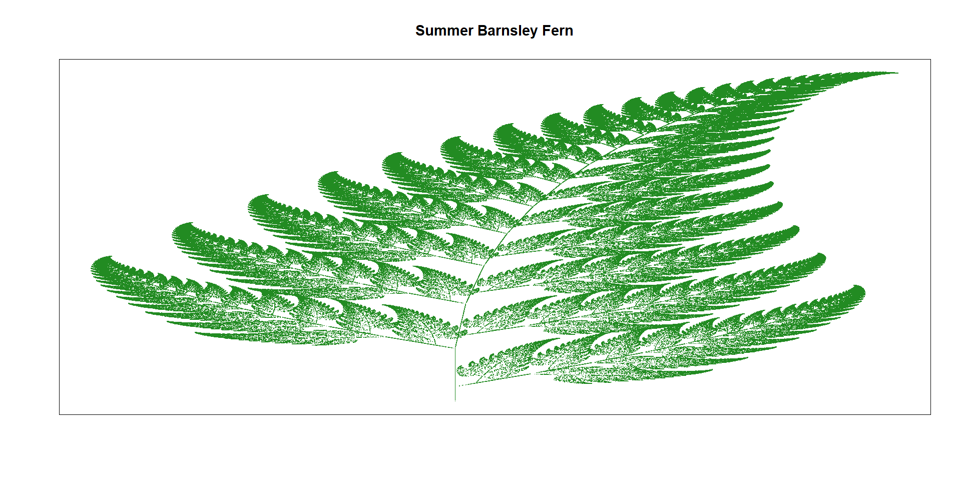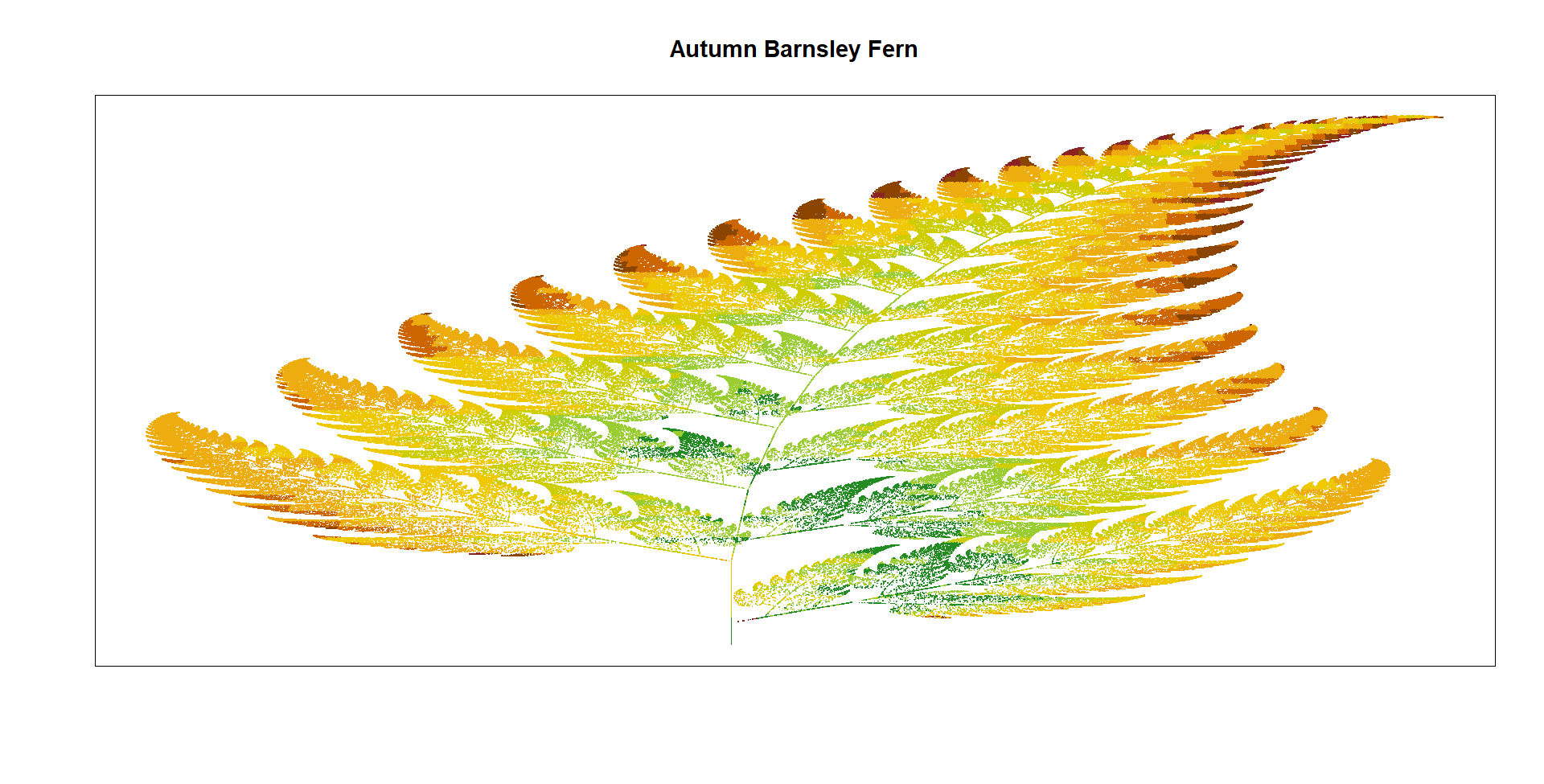df$col <- NA for (r in 1:nrow(color_table) ){ df$col[df$xdev + (df$y/10) <= color_table$value[r] & is.na(df$col)] <- color_table$color[r] } plot(df$x, df$y, pch = '.', col = df$col,xaxt = "n", yaxt = "n", xlab = NA, ylab = NA, main = "Autumn Barnsley Fern") ``` ::: {layout-ncol="2"} ![](Barnsley%20Fern.jpg) ![](autumn-Barnsley%20Fern.jpg) ::: # 4 Brief About Fractal Flame Algorithm Iterated function systems can be a lot more elaborate than the Barnsley fern, often involving transformation functions that are constructed according to some fancypants compositional rules. For example, the [fractal flame algorithm](https://en.wikipedia.org/wiki/Fractal_flame) proposed by Scott Draves in 1992 (here's [the original article](https://flam3.com/flame_draves.pdf)) specifies transformation functions $f_i()$ -- called "flame functions" -- that are composed according to the rule: $$ f_i(\textbf{x}) = \sum_j w_{ij} g_j(\textbf{A}_i \textbf{x}) $$ - $\textbf{A}_i$ is a matrix that defines an affine transformation of the coordinates $\textbf{x}$ associated with this specific flame function (i.e., each flame function $f_i()$ has its own transformation , and in the two dimensional case $\textbf{x}$ is just the points $(x,y)$ ); - The various $g_j()$ functions are called "variant functions", and these don't have to be linear: they can be sinusoidal, or discontinuous, or whatever you like really; - Each flame function is defined as a linear combination of the variant functions: the coefficient $w_{ij}$ specifies the weight assigned to the $j^{\ \text{th}}$ variant function by the $i^{\ \text{th}}$ flame function. Moreover, analogous to the observations made in the context of the Barnsley fern, it is noteworthy that the flame functions can undergo a nuanced refinement through the incorporation of a probability vector. This introduces a sophisticated layer to the system, allowing for the definition of a bias towards certain flame functions over others. In this nuanced extension, the algorithm can be imbued with a probabilistic framework, wherein each flame function is assigned a weight based on a probability distribution. Consequently, during the generation process, certain flame functions are more likely to be invoked, introducing a deliberate emphasis on specific visual characteristics. This introduces a level of control and finesse to the output, enabling the artist or programmer to steer the algorithm towards the realization of desired aesthetic nuances within the generated visualizations. Moreover, akin to the observations elucidated in the context of the Barnsley fern, it is noteworthy that the flame functions, denoted as $f_i(x)$, can undergo a nuanced refinement through the incorporation of a probability vector $\textbf{P}$. This introduces a sophisticated layer to the system, allowing for the definition of a bias towards certain flame functions over others. In this refined model, the algorithm can be imbued with a probabilistic framework, wherein each flame function is assigned a weight based on a probability distribution: $\textbf{P}=(p_1,p_2,…,p_n)$, where $p_i$ represents the probability associated with the $i^{\ \text{th}}$ flame function. Consequently, during the generation process, the invocation of each flame function follows a probabilistic distribution, emphasizing certain functions over others. This deliberate modulation introduces a level of control and finesse to the output, empowering the artist or programmer to steer the algorithm towards the realization of desired aesthetic nuances within the generated visualizations. In the initial stages of foray into the implementation of the fractal flame algorithm, a deliberate choice was made to eschew the integration of nuanced weighting variables denoted by $w_{ij}$. These elements were purposefully neglected. Subsequently, due to a confluence of fatigue and a lapse in meticulous attention to the subscripts embedded within *Draves' equations*, a determination was reached to construct a system wherein each unique combination of a transformation matrix $\textbf{A}_i$ and a variant function $g_j()$ would be accommodated by an individual flame function. The outcome of this deliberation materialized in the form of the ensuing code. Given a set of variant functions $g_1, g_2, \ldots, g_n$, and an ensemble of transformation matrices $\textbf{A}_1,\textbf{A}_2, \ldots,\textbf{A}_m$, the implementation involved the inclusion of every transformation function $f_{ij}(\textbf{x})$ according to the stipulated format: $$ f_{ij}(\textbf{x}) = g_i(\textbf{A}_i\textbf{x}) $$ In orchestrating these transformation functions in the described fashion, the act of sampling a random transformation, denoted as $f_{ij}$, is facilitated by an independent sampling procedure applied to its dual components. This involves the sequential sampling of a transformation matrix $\textbf{A}_i$ and a variant function $g_j$. The process culminates at this juncture. This distinctive approach represents a peculiar yet intriguing variant within the broader context of the fractal flame algorithm. Despite its departure from conventional methodologies, it unfolds as a nuanced pathway that yields aesthetically pleasing outcomes. This unique interplay of independently sampled transformation elements, involving both matrix and function, contributes to the algorithm's versatility, showcasing its capacity to produce visually compelling and intricate visualizations. Now, we will see some computer generated fractal frame art where the coefficients that define the affine transformations $\textbf{A}_i$ have been sampled uniformly at random, with values ranging from $-1$ to $1$. ```{r,warning=FALSE,message=FALSE} unboxer_base <- function(iterations, layers, seed = NULL) { if(!is.null(seed)) set.seed(seed) # coefficients defining affine layer transforms, A_i coeffs <- array( data = runif(9 * layers, min = -1, max = 1), dim = c(3, 3, layers) ) # list of variant functions, g_j funs <- list( function(point) point + (sum(point ^ 2)) ^ (1/3), function(point) sin(point), function(point) 2 * sin(point) ) # updater function: apply the layer, then the function # (the weirdness with point[3] is me treating colour as special) update <- function(point, layer, transform) { f <- funs[[transform]] z <- point[3] point[3] <- 1 point <- f(point %*% coeffs[,,layer]) point[3] <- (point[3] + z)/2 return(point) } # initial point point0 <- matrix( data = runif(3, min = -1, max = 1), nrow = 1, ncol = 3 ) # sample points layer_ind <- sample(layers, iterations, replace = TRUE) trans_ind <- sample(length(funs), iterations, replace = TRUE) points <- accumulate2(layer_ind, trans_ind, update, .init = point0) # tidy up, add columns, and return points <- matrix(unlist(points), ncol = 3, byrow = TRUE) points <- cbind( points, c(0, layer_ind), c(0, trans_ind) ) return(points) } ``` There are three variant functions $g_j$ in this system: two of them are sinusoidal functions: one of them computes $\sin(x)$ and $\sin(y)$, and the other computes the same thing but multiplies the output by two. Both of these will produce wavy shapes. The other one is a re-scaling function: it tends to shift points towards the top right corner. At this juncture, it becomes crucial to introduce and underscore the integration of computer-generated values into the current discourse. This introduces a nuanced layer of complexity and sophistication, signifying a pivotal addition that warrants comprehensive elucidation. In essence, these computer-generated values, integral to the ongoing discussion, play a pivotal role in shaping the trajectory of our inquiry. Their introduction broadens the scope of our exploration, infusing a sophisticated computational dimension that merits detailed consideration. These values, emanating from the computational domain, serve as essential elements that contribute to the intricacies of our analysis. Their incorporation into the narrative not only expands the conceptual framework but also establishes a foundation for subsequent discussions on the interplay between theoretical constructs and computational outcomes. ```{r,eval=FALSE,warning=FALSE,message=FALSE,results='hide'} unboxer_base(10, layers = 5, seed = 333) ``` The first column is the x-coordinate and the second column is the y-coordinate. The third column is a "*z-coordinate*" that we'll map to the colour aesthetic later. Column four specifies the layer number (i.e., the value $i$ specifying which affine matrix $\textbf{A}_i$ was used), and column five specifies the variant function number (i.e., the value $j$ specifying which variant function $g_j$ was used). To transform these numerical values into a visually appealing representation with associated colors, the implementation of a palette function becomes necessary. ```{r,eval=FALSE,warning=FALSE,message=FALSE,results='hide'} sample_canva2 <- function(seed = NULL, n = 4) { if(!is.null(seed)) set.seed(seed) sample(ggthemes::canva_palettes, 1)[[1]] |> (\(x) colorRampPalette(x)(n))() } ``` After completing the aforementioned steps, the rendering function, albeit straightforward, serves its purpose effectively. It comprises basic `ggplot2` code to generate a scatter plot from the points, with coloration applied using a Canva palette: ```{r,eval=FALSE,warning=FALSE,message=FALSE,results='hide'} unbox_art <- function(data, seed = NULL, size = 1) { # convert to data frame and sample a palette data <- data |> as.data.frame() |> as_tibble() names(data) <- c("x", "y", "c", "l", "t")[1:ncol(data)] shades <- sample_canva2(seed) # render image as a scatter plot ggplot(data, aes(x, y, colour = c)) + geom_point( size = size, stroke = 0, show.legend = FALSE ) + theme_void() + coord_equal(xlim = c(-4, 4), ylim = c(-4, 4)) + scale_colour_gradientn(colours = shades) + scale_x_continuous(expand = c(0, 0)) + scale_y_continuous(expand = c(0, 0)) + theme(panel.background = element_rect( fill = shades[1], colour = shades[1] )) } ``` Indeed, the aesthetic appeal is notably enhanced when a substantial number of points, such as 3 million, are generated and plotted with a diminutive marker size, e.g., 0.1. This approach not only accentuates the intricacies of the rendered fern but also contributes to a visually striking and finely detailed representation. The combination of a large dataset and a small marker size serves to amplify the artistic quality and overall visual impact of the generated plot. ```{r,eval=FALSE,warning=FALSE,message=FALSE,results='hide'} mil <- 1000000 tic() unboxer_base(3 * mil, layers = 3, seed = 66) |> unbox_art(seed = 66, size = .1) ``` ![](artfractal-frame.jpg){fig-align="center" width="499"} The computational efficiency of the system is moderate. Nevertheless, we will discuss shortly the implementation of measures to notably expedite this process. ```{r,eval=FALSE,warning=FALSE,message=FALSE,results='hide'} tic() unboxer_base(mil, layers = 2, seed = 999) |> unbox_art(seed = 2, size = .2) unboxer_base(mil, layers = 5, seed = 333) |> unbox_art(seed = 2, size = .2) unboxer_base(mil, layers = 9, seed = 420) |> unbox_art(seed = 2, size = .2) toc() ``` ::: {layout-ncol="2"} ![](art-creative.jpg) ![](frac-algo-art.jpg) ::: ![](plot.jpg){fig-align="center" width="601"} The outputs from this system exhibit a consistent visual motif: a pair of nested boxes with an emergent element emanating from the top-right corner. While the broad structure remains uniform, the finer details exhibit substantial variation across different outputs. Notably, there are discernible systematic differences contingent on the number of layers employed. The provided example illustrates the impact on the output as the number of layers progresses incrementally from 2 to 9, revealing a nuanced evolution in the complexity and intricacy of the generated patterns. To comprehend the dynamics of this system, we will undertake a similar approach as we did with the Barnsley fern. we will generate the data for an artwork by invoking **`unboxer_base()`**, followed by three distinct visualizations. Initially, we will present a pure black and white image to elucidate the overall arrangement of points. Subsequently, we will deconstruct it based on the components. Given that each transformation function is delineated in terms of the affine and variant components, we will provide two distinct versions to elucidate these aspects. ```{r,eval=FALSE,warning=FALSE,message=FALSE,results='hide'} dat <- unboxer_base(mil, layers = 2, seed = 99) |> as.data.frame() |> as_tibble() names(dat) <- c("x", "y", "c", "affine_layer", "variant_function") dat <- dat |> slice_tail(n = -1) |> mutate( affine_layer = factor(affine_layer), variant_function = factor(variant_function) ) ggplot(dat, aes(x, y)) + geom_point(size = .4, stroke = 0, show.legend = FALSE) + theme_void() + coord_equal(xlim = c(-4, 4), ylim = c(-4, 4)) ggplot(dat, aes(x, y, colour = variant_function)) + geom_point(size = .4, stroke = 0) + coord_equal(xlim = c(-4, 4), ylim = c(-4, 4)) + scale_colour_brewer(palette = "Set2") + guides(colour = guide_legend(nrow = 1, override.aes = list(size = 5))) + theme_void() + theme(legend.position = c(0.2, 0.1)) ggplot(dat, aes(x, y, colour = affine_layer)) + geom_point(size = .4, stroke = 0) + coord_equal(xlim = c(-4, 4), ylim = c(-4, 4)) + scale_colour_brewer(palette = "Set1") + guides(colour = guide_legend(nrow = 1, override.aes = list(size = 5))) + theme_void() + theme(legend.position = c(0.2, 0.1)) ``` ::: {layout-ncol="2"} ![](flame-fractal.jpg) ![](frac.jpg) ::: ![](art-of-fractals.jpg){fig-align="center" width="650"} This comprehensive analysis affords a profound understanding of the intricate processes at play within the depicted visuals. Focusing on the central panel, the observable manifestation of geometric patterns is inherently tied to the influence exerted by the two distinct "sinusoidal" components. The key to this phenomenon lies in the inherent constraints of the sine function, which, confined within the range of -1 to 1, gives rise to the formation of discernible boxes. However, it is imperative to note that the intricate, undulating patterns apparent in select outputs bear an inherent relationship with these sinusoidal components, although the graphical representation may not overtly elucidate this nuanced association. In deliberate contrast, the panel situated on the right of the visual display unveils a lucid portrayal of the transformative impact arising from the application of affine transformations. It is particularly noteworthy that the blue pattern assumes a semblance to a "squashed and rotated" rendition of the red pattern. This observation encapsulates the precise function of affine transforms -- introducing deliberate distortions that imbue the generated outputs with a distinctive visual character. This nuanced exploration not only enhances our appreciation of the graphical representations but also serves as a foundation for delving deeper into the intricate interplay of mathematical constructs and visual outcomes. # Conclusion In conclusion, the multifaceted exploration of geometric patterns and visual outcomes, as elucidated through the interplay of sinusoidal components and affine transformations, opens avenues for further research and investigation. This preliminary analysis provides a foundational understanding of the underlying dynamics, shedding light on the constraints imposed by mathematical functions and the transformative potential inherent in affine operations. To propel this inquiry forward, a promising avenue for future research involves a more granular examination of the nuanced relationships between specific mathematical components and their visual manifestations. Exploring the potential variations in constraints, modifying parameters, or introducing additional elements could unearth deeper insights into the rich tapestry of geometric patterns generated through computational processes. Furthermore, an in-depth exploration of the role of probability vectors, as mentioned earlier, could serve as a catalyst for advancing the sophistication of these generative algorithms. Investigating the impact of weighted probabilities on the prevalence of certain visual features could contribute to the refinement of aesthetic control in the output. Additionally, considering the broader implications of these generative processes, both from an artistic and mathematical standpoint, opens up interdisciplinary avenues. Collaborations between mathematicians, artists, and computer scientists could foster innovative approaches, leading to the creation of visually compelling outputs that not only adhere to mathematical principles but also push the boundaries of artistic expression. In essence, the presented analysis lays the groundwork for a more intricate exploration of generative algorithms, paving the way for future investigations that delve deeper into the mathematical intricacies and artistic potential inherent in these computational systems. The journey towards unraveling the full extent of these generative capabilities promises to be both challenging and rewarding, offering rich opportunities for interdisciplinary collaboration and creative exploration. # **Footnotes** - [The Fractal Flame Algorithm](https://flam3.com/flame_draves.pdf) - [Sierpiński triangle](https://en.wikipedia.org/wiki/Sierpi%C5%84ski_triangle) - [Chaos Game](https://en.wikipedia.org/wiki/Chaos_game) # References 1. [Fractals Everywhere](https://books.google.com/books?id=oh7NoePgmOIC), Boston, MA: Academic Press, 1993, [ISBN](https://en.wikipedia.org/wiki/ISBN_(identifier) "ISBN (identifier)") [0-12-079062-9](https://en.wikipedia.org/wiki/Special:BookSources/0-12-079062-9 "Special:BookSources/0-12-079062-9") 2. <https://flam3.com/flame_draves.pdf> 3. [Falconer, Kenneth](https://en.wikipedia.org/wiki/Kenneth_Falconer_(mathematician) "Kenneth Falconer (mathematician)") (1990). [*Fractal geometry: Mathematical foundations and applications*](https://archive.org/details/fractalgeometrym0000falc/page/113). John Wiley and Sons. pp. [113--117, 136](https://archive.org/details/fractalgeometrym0000falc/page/113). [ISBN](https://en.wikipedia.org/wiki/ISBN_(identifier) "ISBN (identifier)") [0-471-92287-0](https://en.wikipedia.org/wiki/Special:BookSources/0-471-92287-0 "Special:BookSources/0-471-92287-0"). 4. [Barnsley, Michael](https://en.wikipedia.org/wiki/Michael_Barnsley "Michael Barnsley"); Andrew Vince (2011). "The Chaos Game on a General Iterated Function System". *Ergodic Theory Dynam. Systems*. **31** (4): 1073--1079. [arXiv](https://en.wikipedia.org/wiki/ArXiv_(identifier) "ArXiv (identifier)"):[1005.0322](https://arxiv.org/abs/1005.0322). [Bibcode](https://en.wikipedia.org/wiki/Bibcode_(identifier) "Bibcode (identifier)"):[2010arXiv1005.0322B](https://ui.adsabs.harvard.edu/abs/2010arXiv1005.0322B). [doi](https://en.wikipedia.org/wiki/Doi_(identifier) "Doi (identifier)"):[10.1017/S0143385710000428](https://doi.org/10.1017%2FS0143385710000428). [S2CID](https://en.wikipedia.org/wiki/S2CID_(identifier) "S2CID (identifier)") [122674315](https://api.semanticscholar.org/CorpusID:122674315). 5. [Draves, Scott](https://en.wikipedia.org/wiki/Scott_Draves "Scott Draves"); Erik Reckase (July 2007). ["The Fractal Flame Algorithm"](https://web.archive.org/web/20080509073421/http://flam3.com/flame.pdf) (PDF). Archived from [the original](http://flam3.com/flame.pdf) (PDF) on 2008-05-09. Retrieved 2008-07-17. 6. Dietmar Saupe, Raouf Hamzaoui. ["A Review of the Fractal Image Compression Literature"](https://www.uni-konstanz.de/mmsp/pubsys/publishedFiles/SaHa94.pdf) 7. Bauschke, Heinz H. (2017). *Convex Analysis and Monotone Operator Theory in Hilbert Spaces*. New York: Springer.