Exploring the Realm of Uncertainty
Navigating Deterministic and Indeterministic Realms
Why Probability?
Uncertainty, the profound mystery inherent in our universe, eludes precise understanding. A perpetual game unfolds—the ‘Game of Chances.’ Amidst deterministic and indeterministic processes, a novel concept emerges: ‘Probability.’ Our pursuit is to discern patterns within chaos. In this context, let us engage in a game that unveils the essence of probability and its overarching objective.
Unraveling the Game
Assume a particle is located at the origin, i.e., at \((0, 0)\) of a two-dimensional Euclidean plane. Consider a die with four sides denoted by the integers \(1, 2, 3, 4\). The particle moves on the plane according to rules as shown in Table 1: Initially, the particle is at \((0, 0)\); now, imagine \(2\) shows up after
| A number appears in the dice | Where the particle moves |
|---|---|
| 1 | \((0.8x+0.1, 0.8y+0.04)\) |
| 2 | \((0.6𝑥 +0.19, 0.6𝑦 +0.5)\) |
| 3 | \((0.466(𝑥 -𝑦)+0.266, 0.466(𝑥 +𝑦)+0.067)\) |
| 4 | \((0.466(𝑥 +𝑦)+0.456, 0.466(y-x)+0.434)\) |
throwing the die. From the rules described in the table, the particle will move to \((0.6𝑥 +0.19, 0.6𝑦 +0.5)\) where \((𝑥, 𝑦)\) is its current coordinate. For us, \((𝑥, 𝑦) = (0,0) = 𝑋_0\) the initial position of the particle, and since \(2\) has appeared, the next position or co-ordinate of the particle is the initial position of the particle, and since \(2\) has appeared, the next position or co-ordinate of the particle is,
\[ (0.6\times 0 + 0.19, 0.6 \times 0 + 0.5) = (0.19,0.5)=X_1 \]
We mark the point \((0.19,0.5)\) with a pen. We throw the die again, and depending on the number, and the particle moves to a different point from \((0.19, 0.5)\). If we repeat these steps for, say, \(20, 000\) times (Of course, that requires the help of a computer) and mark those points on the plane, we get a picture similar to figure below.
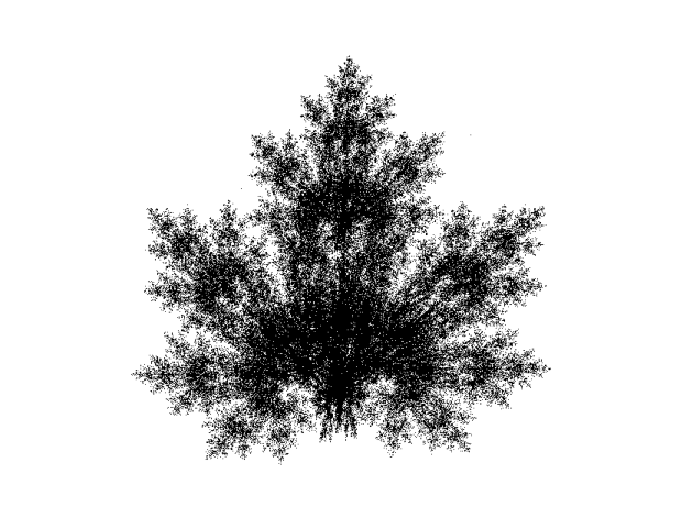
The particle’s random visits to points on a leaf’s surface are insufficient to cover all locations and form a complete, naturally shaped leaf without holes. After multiple iterations, the particle settles into a single position on a two-dimensional maple leaf, referred to as its accessible position. Demonstrably, the sequence of points in the particle’s trajectory will, with probability one, pass through any portion of the Maple leaf. Despite the randomness of individual steps, the long-term behavior of the movement remarkably takes on the distinct shape of a Maple leaf. This outcome remains consistent regardless of the number of players or iterations. Emphasis is placed on the concept of “with probability one,” which will be clarified later. The trajectory approaches the same point if a dice consistently shows the same face, but for a fair dice, this is highly improbable. The continual tossing of the dice is termed “iteration,” and the rule governing the particle’s advancement is known as a “function.” Notably, the four rules in the table can be viewed as specific functions.\(w_1,w_2,w_3,w_4\) acting on \(\begin{bmatrix}x\\y\end{bmatrix} \in \mathbb{R}^2\) as follows:
\[ w_1\Bigg(\begin{bmatrix}x\\y\end{bmatrix}\Bigg)= \begin{bmatrix} 0.8 & 0 \\ 0 & 0.8 \end{bmatrix} +\begin{bmatrix}x\\y\end{bmatrix}+ \begin{bmatrix} 0.1\\0.04\end{bmatrix} \]
\[ w_2\Bigg(\begin{bmatrix}x\\y\end{bmatrix}\Bigg)= \begin{bmatrix} 0.6 & 0 \\ 0 & 0.6 \end{bmatrix} +\begin{bmatrix}x\\y\end{bmatrix}+ \begin{bmatrix} 0.19\\0.5\end{bmatrix} \]
\[ w_3\Bigg(\begin{bmatrix}x\\y\end{bmatrix}\Bigg)= \begin{bmatrix} 0.466 & -0.466 \\ 0.466 & 0.466 \end{bmatrix} +\begin{bmatrix}x\\y\end{bmatrix}+ \begin{bmatrix} 0.266\\0.067\end{bmatrix} \]
\[ w_4\Bigg(\begin{bmatrix}x\\y\end{bmatrix}\Bigg)= \begin{bmatrix} 0.466 & -0.466 \\ 0.466 & 0.466 \end{bmatrix} +\begin{bmatrix}x\\y\end{bmatrix}+ \begin{bmatrix} 0.456\\0.434\end{bmatrix} \]
The chaotic game seen above illustrates the “random repetition of functions” where the randomness appeared due to the throwing of the die. This is absolutely strange where a random process turns into deterministic. So, in terms of probability & statistics, this process is known as statistical regularity.
Motivation and the Achievement in Probability
To understand what we are trying to achieve, and what we are trying to conclude, it is necessary to get introduced to two important words. One has to be clear when he/she is going to use these two words frequently in probabilistic phenomena i.e. Deterministic and Indeterministic.
Deterministic: The word deterministic refers, to a belief that everything that happens must happen as it does and could not have happened any other way. Now, if we say that when a methodology is deterministic it refers that the chance of occurrence of the event involved is ignored and the method used is considered to follow a definite rule. If we make more simplification, deterministic addresses the situation which will take place is already predetermined.
Indeterministic: The word indeterministic refers to the idea that events are not caused deterministically. It is the idea that the will is a free and deliberate choice and actions are not determined by or predictable from antecedent causes.
In our mathematical science, there are two types of experiments — 1) Random Experiment, and 2) Deterministic Experiment.
Deterministic vs Random Experiment
Random Experiment
An experiment is random if it is repeated numerous times under the same conditions.
The outcome of an individual random experiment must be I.I.D. (independent & identically distributed)
Before we carry it out, we cannot predict its outcome.
It can be repeated as many times as we want always under the same conditions.
That means in the case of a random experiment, we know the possible outcomes, but in a particular occurrence, which outcome is going to occur that we cannot predict.
Example:
Percentage of call dropped due to errors over a particular time period. The experiment can yield several different outcomes in the region 0−100%
The time difference between two messages arriving at a message centre. This experiment can yield any number of possible outcomes.
The time difference between two different voice calls over a particular network. This too can yield any number of possible outcomes.
Deterministic Experiment
In a deterministic experiment, the result might be anticipated with assurance in advance, such as the addition of two numbers 5 and 6 or we can say these experiments give the same outcome under identical conditions.
Determining your savings account amount after a month (including your principal amount and the interest amount).
The relationship between a boundary and radius of a circle, or the area and radius of a circle.
That means the set of all possible outcomes is completely determined before carrying it out.
In probability, our aim is to uncover patterns within chaos, particularly in dealing with indeterministic aspects. When observing indeterministic sequences, our interest lies in whether they show behavior akin to deterministic sequences. If an indeterministic sequence closely resembles a deterministic one, it suggests the emergence of a consistent pattern, a noteworthy accomplishment in dealing with inherently unpredictable phenomena. In probability and statistics, our focus centers on understanding and characterizing what is indeterministic and cannot be definitively determined.
The main motive of probability i.e. to make a thorough study on the indeterministic things which are not obvious. We are trying to achieve or learn how to predict things in indeterministic situations i.e., how to predict things where we cannot determine something completely.
The Mystery
We were engaged in the exploration of random phenomena, and the intrigue surrounding these random occurrences lies in the game we were actively participating in. The revelation of this interesting aspect becomes apparent when we alter the system of equations in a specific manner.
| A number appears in the dice | Where the particle moves |
|---|---|
| 1 | \((0,0.16y)\) |
| 2 | \((0.85x-0.04y,-0.04x+0.85y+1.6)\) |
| 3 | \((0.2x-0.26y,0.23x+0.22y+1.6)\) |
| 4 | \((-0.15x+0.28y,0.26x+0.24y+0.44)\) |

When you observe the resulting image, you will notice a difference compared to the previous one. Alternatively, if you choose a different system of equations, you may no longer discern any recognizable pattern.
Indeterministic processes lack complete predictability due to complexity or insufficient information, while randomness denotes events occurring without discernible patterns or order. Randomness is a subset of indeterminism, emphasizing chance and absence of predictability.
Basic Formalism
Now, we shall commence our exploration of mathematical concepts. Deterministic behavior emerges from a random phenomenon when you perform the same random process numerous times under the same condition. In the section ‘Unraveling the Game’, the entirety of random tasks or phenomena within the context of mathematics, probability, and statistics is referred to as a ‘Random Experiment.’ If this random experiment is conducted numerous times under identical conditions, each instance is designated as a ‘Trial’.
Formal Definition
Definition 1.1
Random Experiment
A random experiment refers to a process or activity with an unpredictable outcome. In the context of a coin toss, the experiment involves flipping the coin, and the result (heads or tails) is not precisely known beforehand due to the inherent unpredictability of the coin’s motion.
The randomness in the coin toss arises from factors such as initial conditions (the force and angle of the toss), air resistance, and the nature of the coin’s surface. While the laws of physics govern the motion, the specific outcome is uncertain.
Trial
A trial is a single occurrence of a random experiment. In the context of a coin toss, each flip of the coin constitutes a trial. It involves executing the experiment once and observing the outcome.
Performing multiple trials provides insights into the variability of outcomes. In a coin toss, even under similar conditions, the result may differ due to the inherent randomness. The more trials conducted, the better one can understand the overall behavior and patterns in the experiment.
Example 1
If we toss a fair coin, the possible outcomes are \({\text{Head, Tail}}\). Similarly, when we roll a die once, the potential results are \({1,2,3,4,5,6}\). Now, consider tossing a fair coin twice, leading to outcomes in the set \({\text{(Head, Head), (Head, Tail), (Tail, Head), (Tail, Tail)}}\). Here, \((\text{Head, Tail})\) denotes that the first toss resulted in a Head, and the second in a Tail.
The act of tossing a coin or rolling a die is considered a random experiment. When tossing a fair coin twice, the set of outcomes, \({\text{(Head, Head), (Head, Tail), (Tail, Head), (Tail, Tail)}}\), is known as the sample space. In the first trial, the outcome \(\text{(Head, Head)}\) is a possibility, and in the second trial, \(\text{(Head, Tail)}\) could occur. Thus, the possibilities vary with each trial.
In this context, let us delve into the concept of the sample space. A sample space is formally defined as a set, and its elements represent the possible outcomes derived from a random experiment. In mathematical terminology, these outcomes are referred to as ‘outcomes.’ Due to their nature as elements within the sample space, they are specifically termed ‘sample points.’
Definition 1.2
Sample Space
The sample space, denoted as \(S\), is the set of all possible outcomes of a random experiment. It encompasses every conceivable result that can occur in the experiment.
Example: For a coin toss, the sample space \(S\) would be \(\text{{Heads, Tails}}\). For a six-sided die roll, \(S\) would be \(\{1,2,3,4,5,6\}\).
Sample Point
A sample point, denoted as \(S\), is an individual outcome or element within the sample space. Each sample point represents a specific result of the random experiment.
Example: In the context of a coin toss, individual sample points within the sample space \(\text{\{Heads, Tails\}}\) would be \(\text{\{Heads\}}\) and \(\text{\{Tails\}}\). For a six-sided die, each number \(\{1,2,3,4,5,6\}\) would be a sample point.
The sample space encompasses all possible outcomes, while each outcome within that space is termed a sample point. Together, they form the foundation for understanding and calculating probabilities in a given random experiment.
We frequently discuss the coin toss as a paradigmatic example of a random experiment, a concept integral to probability theory. This holds significant importance and is encapsulated by the term ‘Bernoulli Random Experiment.’ In this context, we represent the outcomes as \(0\) and \(1\) instead of the traditional Head or Tail. However, the fundamental concept remains unchanged.
Bernoulli Trail
Any random experiment with sample space \(\{0,1\}\) is called Bernoulli Random Experiment. A trial of such a random experiment is called a Bernoulli Trial. For example, if we toss a coin and denote “Head” by \(1\) and tail by \(0\) then we got a Bernoulli trial. Similarly, any trial of a random experiment having sample space with seize \(2\), maybe considered as a Bernoulli trial. In the realm of probability and statistics, a pivotal concept emerges—‘Event.’ To elucidate this concept, let us consider an illustrative example.
Example 2
You are tasked with conducting a random experiment involving a fair six-sided die. Your objective is to select a specific sample space, wherein the sum of two dice throws is greater than or equal to \(10\).
Sample Space (\(\Omega\)): \(\{ \text{All possible outcomes}\}\)
\[ \Omega: \{(i,j): i,j =1,\ldots,6\} \]
Here we’re interested a special subset. We’re interested in \(\displaystyle \Bigg\{(i,j) \in \Omega: i+j\ge 10\Bigg\}\). So from your original sample space is now known to you & under certain condition you’ve to construct a subset of your sample space i.e., \(\{(4,6),(5,5),(5,6),(6,4),(6,5),(6,6)\}\) this is your subset. In terms of probability & statistics, it’s known as Event.
Girolamo Cardano is actually the first person known to invent probability. However his work was not published until centuries later and during that time the letters were exchanged and probability was born. Cardano was an Italian professor of mathematics and medicine, as well as an avid gambler; he gambled daily. He felt that if he wasn’t going to win money, then he could be doing something more worthwhile such as learning. This idea led him to investigate the chances of pulling aces out of a deck of cards and also rolling sevens with two dice. He was the first to realize that there was the same chance to roll a 1,3, or 5 as there was to roll a 2, 4, or 6. People would then bet accordingly if the dice were fair. If the dice were not fair, then the bets would need to be moved to accommodate for that. He was also the first to discover the idea of counting the number of favorable cases (successes) and comparing them to the total number of cases, and he wanted to assign a number from 0 to 1 to the probability of an outcome (Jardine, 2000).
In this context let’s give you another example from a gambling perspective. So, game is like this,
Example 3
In a series of \(10\) die throws, an individual is deemed victorious or defeated based on whether the sum surpasses \(24\).
The creator of this game has had an intuitive experience—specifically, a previous loss. Consequently, there is a keen desire for precision in measurement. Given the potential financial implications associated with losing the game, clarity becomes paramount. To achieve such precision, mathematical assistance is sought, and herein lies the relevance of probability.
\[ \Omega: \{ (1,2,1,2,3,4,6,5,6,3) \ldots\} \]
Here, we are interested a special subset. We’re interested in \(\displaystyle\Bigg\{x \in\Omega: \sum_{i=1}^{10} x_i \ge 24\Bigg\}\). In other words, all those elements \(x_i\) inside this sample space such that sum of those elements is greater than equal to \(24\); where \(x\)’s are my throw values. Therefore,
\[\Bigg\{x \in\Omega: \sum_{i=1}^{10} x_i \ge 24\Bigg\} = \text{Event} \subseteq \Omega\]
This the concept behind the Event. Let’s introduce by a formal definition.
Definition 1.3
Event
An event is a subset of the sample space of a random experiment. It comprises one or more outcomes that can occur when the experiment is performed. Events are used to describe and analyze specific occurrences or results within the overall set of possible outcomes.
Example: Consider rolling a six-sided die. The sample space, \(S\), is \(\{1,2,3,4,5,6\}\). An event, such as obtaining an even number, would be represented as \(E=\{2,4,6\}\), where \(E\) is the event of rolling an even number.
In this context, there is a subtle but crucial issue to consider. While events are defined as subsets of the sample space, the reverse may not always be true—some subsets of the sample space may not qualify as events. This complexity is beyond the scope of detailed discussion here. The practical subsets used in daily work are exclusively events, and this distinction is essential for understanding the subsequent problem. Referring to these subsets collectively as the event space,it’s noteworthy that the nomenclature varies, commonly known as a sigma field or sigma-algebra in international literature. Regardless of the terminology used, the fundamental definition remains consistent—an event is a concise list of what we conceptualize as natural occurrences. This clarification is essential for the subsequent problem.
Let a random experiment have sample space \(S\). Then by the event space of the random experiment, we mean a collection \(\mathscr{F}\) of subsets of \(S\) satisfying the following conditions
\(S \in \mathscr{F}\;\;\big( \text{Entire sample space itself an event}\big)\)
\(\forall A \in \mathscr{F,} \; A^c \in \mathscr{F}\) The compliment of an event is an event also, if occurring ‘Head’ is an event then occurring ‘tail’ is an event also.
\(\displaystyle\forall A_i \in \mathscr{F}; \forall\ i=1(1)n \; \;\bigcup_{i=1}^{n} A_i \in \mathscr{F}\)
These conditions also imply that \(\mathscr{F}\) is closed under countable intersection. The elements of \(\mathscr{F}\) are called events.
Now, let us consider an illustrative example. Through this, you will gain a precise understanding of the aforementioned theory.
Example 4
\(\text{If}\; S = \{0,1\}\; \text{then}\; \mathscr{F}_1=\{\phi,\{0,1\}\}\; \text{is one possible event space.}\; \mathscr{F}_2=\{\phi,\{0\},\{1\},\{0,1\}\}\) \(\text{is another. But}\; \mathscr{F}_3 = \{\{0\},\{1\}\}\; \text{is not. Because,}\; A_1=\{0\}\; \text{and}\; A_2= \{1\}\; \text{third condition}\) \(\text{is not satisfying. Therefore,}\; A_1,A_2 \in\mathscr{F_3}\; \text{but}\; A_1\cup A_2 \notin \mathscr{F_3}.\)
However, for a finite sample space \(S,\) the most common choice for event space, the most common choice for event space is the power set \(\mathscr{P}(S).\)
Now that we have acquired a wealth of new terminology, let us redirect our focus to the concept of statistical regularity. In the context of random experiments involving events, the objective is to discern an inherent statistical regularity within the experiment. These random experiments are conducted iteratively, as exemplified by the recurrent act of tossing a coin. Consider an event, such as the occurrence of a ‘head’ during each toss. Subsequent to each instance of this event, document whether it transpired. To elucidate, contemplate the initial five toss results:
\[ \text{Head, Tail, Head, Head, Tail. } \]
To appraise the frequency of ‘heads’ after each toss, a cumulative count is meticulously maintained. These counts represent the incidence of ‘heads’ in the sequence. Following the first toss, the frequency is 1, as a ‘head’ was obtained. Subsequently, after the second toss, the frequency remains at 1, given that the second toss resulted in a ‘tail,’ and so forth. If tabulated, this information can be presented as follows:
| Number of Toss(n) | 1 | 2 | 3 | 4 | 5 |
|---|---|---|---|---|---|
| Outcome | Head | Tail | Head | Head | Tail |
| Frequency | 1 | 1 | 2 | 3 | 3 |
Now, let us examine the ratio of occurrences of obtaining a ‘head’; this involves dividing the number of ‘head’ outcomes by the total number of tosses. Consequently, I will refer to this ratio as the relative frequency. For instance, following the first toss, where a ‘head’ was obtained once, the frequency of ‘head’ is 1. The denominator, representing the total number of tosses, remains 1. Therefore, the relative frequency is equal to 1. After the second toss, the observation reveals that out of 2 tosses, 1 resulted in a ‘head.’ Consequently, the relative frequency is expressed as \(1/2\). This pattern persists for subsequent tosses. If presented in tabular form–
| Number of Toss(n) | 1 | 2 | 3 | 4 | 5 |
|---|---|---|---|---|---|
| Outcome | Head | Tail | Head | Head | Tail |
| Frequency | 1 | 1 | 2 | 3 | 3 |
| Relative Frequency | 1 | \(\frac{1}{2}\) | \(\frac{2}{3}\) | \(\frac{3}{4}\) | \(\frac{2}{5}\) |
In this particular example, we conducted 5 tosses. Consider the scenario where this process is repeated numerous times, for instance, \(300\) times. If we were to depict the results graphically, with the number of tosses (n) represented on the x-axis and the corresponding relative frequency on the y-axis, the resulting graph undoubtedly takes on a random appearance. I have illustrated such a graph in Fig-3 below.
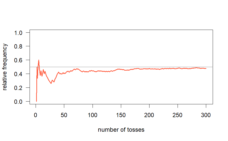
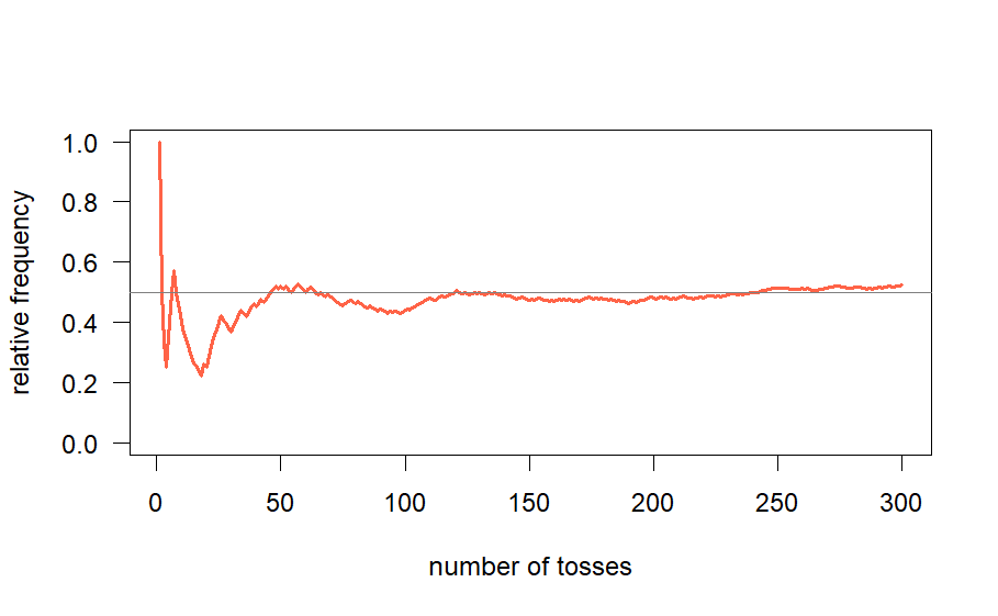
The graph initially exhibits irregularities, followed by a gradual reduction in randomness, leading to the emergence of a horizontal straight line. Conducting additional sets of 300 coin tosses yields different initial outcomes, but they eventually converge into identical horizontal lines. Despite apparent graphical disparities, increasing the number of tosses diminishes these differences. This consistent pattern of initial irregularities and subsequent convergence towards a specific value is a fundamental principle substantiated numerically, forming the basis of probability theory and statistics. This concept, inspired by Ludo’s images of maple and fern leaves, involves intricate mathematics, ultimately representing a variant of the overarching problem. The graph tends to stabilize as it approaches a critical point, demonstrating a consistent pattern reminiscent of an enchanted snake. This behavior is encapsulated by the term ‘probability.’ An event, representing a significant occurrence, is associated with a sample space and an underlying random experiment. Repeating this experiment and graphing the relative frequency of the event consistently converges to a specific value, termed the magic number—the probability of the event.
What is Statistical Regularity?
The accuracy of results hinges on independently conducting each random experiment. Repeating the same experiment using prior data does not ensure consistency, as the resulting graph may exhibit unpredictability or shift across different domains. Independence, a crucial concept, means that the outcome of one trial does not affect subsequent trials. This principle, discussed further in this chapter, emphasizes that each trial must be executed afresh.
Q. What is meant by the term “statistical regularity”? Explain how the frequency definition of the probability of a random event is related to the concept of statistical regularity.
Statistics deals with random experiments. The outcome of a random experiment may not be known for sure in advance, unlike deterministic mathematics (e.g., \(2+3 = 5\)). Thus, we may think of randomness as “’irregularity”. However, in certain situations, even outcomes of random experiments show a regularity that is similar to deterministic behaviour. This is called statistical regularity:
If the same random experiment is repeated independently for a large number of times then certain aggregate behaviours of the outcomes often converge to a deterministic number.
The term ‘aggregate behavior’ may seem concise; let us elaborate. In this context, it refers to the compilation of exam marks, signifying the total across all subjects. Additionally, ‘aggregate’ pertains to the cumulation of all trials conducted thus far, combining outcomes to form a collective number. For instance, in the scenario of repeated coin tosses, the relative frequency is calculated based on the cumulative number of tosses conducted up to a given point.
For example, if a coin is tossed times then the relative frequency of heads approaches a fixed number as \(n \to \infty\) . Such regular behaviours can be proved using various theorems of probability.
Frequency Definition of Probability: Frequency definition of probability”: Suppose that we have a random experiment with sample space \(S\). Let \(A\subseteq S\) be any event. Let us repeat the random experiment times independently. Let \(X_n\) = the relative frequency of the event during these trials.
Then it is seen that as \(n \to \infty\) the random variable \(X_n\), approaches some fixed number. This behaviour is an example of statistical regularity. The limiting fixed number is called the probability of the event. This is called the “frequency definition of probability”.
The term I previously mentioned as a ‘definition’ is not a mathematical definition. To formulate a mathematical definition based on statistical regularity, it is imperative to substantiate the concept with numerical evidence. This substantiation relies on the use of probability. Paradoxically, this leads to a circular dependency, as probability is invoked to define probability.
However, there is a definitive mathematical definition for probability known as the axiomatic definition, which will be explored in the subsequent discussion. This eliminates the ‘egg first, chicken first’ dilemma. The significance of the ’frequency definition of probability’ remains evident, emphasizing the ease with which the concept of probability can be comprehended through the lens of statistical regularity.
See Also
References
Probability & Statistics by Arnab Chakraborty
Iterated Function Systems: A comprehensive Survey by Ramen Ghosh , Jakub Marecek