Classical Theory of Probability

Probability Theory Using R

Sample Spaces and Pebble World

The mathematical framework for probability is built around sets. Imagine that an experiment is performed, resulting in one out of a set of possible outcomes. Before the experiment is performed, it is unknown which outcome will be the result; after, the result “crystallizes” into the actual outcome.

Definition

Sample space and event: The sample space \(S\) of an experiment is the set of all possible outcomes of the experiment. An event \(A\) is a subset of the sample space \(S\), and we say that \(A\) occurred if the actual outcome is in \(A\).

A sample space as Pebble World, with two events A and B spotlighted.

The sample space of an experiment can be finite, countably infinite, or uncountably infinite. When the sample space is finite, we can visualize it as Pebble World, as shown in Figure above. Each pebble represents an outcome, and an event is a set of pebbles. Performing the experiment amounts to randomly selecting one pebble. If all the pebbles are of the same mass, all the pebbles are equally likely to be chosen.

Here we give a general definition of probability that allows the pebbles to differ in mass. Set theory is very useful in probability since it provides a rich language for expressing and working with events;

For example, let \(S\) be the sample space of an experiment and let \(A,B \subseteq S\) be events. Then the union \(A \cup B\) is the event that occurs if and only if at least one of \(A\) and \(B\) occurs, the intersection \(A \cap B\) is the event that occurs if and only if both \(A\) and \(B\) occur, and the complement \(A^c\) is the event that occurs if and only if \(A\) does not occur. We also have De Morgan’s laws:

\[ (A \cup B)^c = A^c \cap B^c\; \text{and}\; (A \cap B)^C = A^c \cup B^c \]

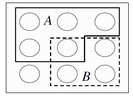
since saying that it is not the case that at least one of \(A\) and \(B\) occur is the same as saying that \(A\) does not occur and \(B\) does not occur, and saying that it is not the case that both occur is the same as saying that at least one does not occur. Analogous results hold for unions and intersections of more than two events. In the example shown in figure above, \(A\) is a set of \(5\) pebbles, \(B\) is a set of \(4\) pebbles, \(A \cup B\) consists of the \(8\) pebbles in \(A\) or \(B\) (including the pebble that is in both), \(A \cap B\) consists of the pebble that is in both A and \(B\), and \(A^c\) consists of the \(4\) pebbles that are not in \(A\). The notion of sample space is very general and abstract, so it is important to have some concrete examples in mind.

Naive Definition of Probability

Historically, the earliest definition of the probability of an event was to count the number of ways the event could happen and divide by the total number of possible outcomes for the experiment. We call this the naive definition since it is restrictive and relies on strong assumptions; nevertheless, it is important to understand, and useful when not misused.

Definition:

Naive definition of probability: Let \(A\) be an event for an experiment with a finite sample space \(S\). The naive probability of \(A\) is

\[ P _{Naive}(A) = \dfrac{|A|}{|S|} = \dfrac{\text{No. of outcomes favourable in A}}{{\text{Total number of outcomes in S}}} \]

\(|A|\) to denote the size of \(A\);

In terms of Pebble World, the naive definition just says that the probability of \(A\) is the fraction of pebbles that are in \(A\). For example, in figure it says,

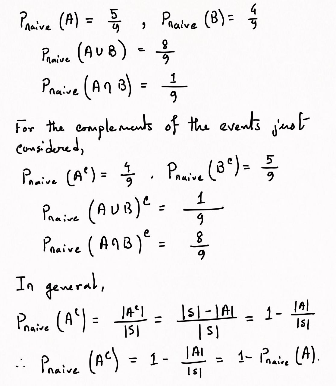
A good strategy when trying to find the probability of an event is to start by thinking about whether it will be easier to find the probability of the event or the probability of its complement. The naive definition is very restrictive in that it requires \(S\) to be finite, with equal mass for each pebble. It has often been misapplied by people who assume equally likely outcomes without justification and make arguments to the effect of “either it will happen or it won’t, and we do not know which, so it’s \(50-50\)”.

In this ‘Elementary Probability Using R’ let you try out some of the examples from the chapter, especially via simulation.

Counting Rules Using R

Vectors

R is built around vectors, and getting familiar with “vectorized thinking” is very important for using R effectively. To create a vector, we can use the c() command (which stands for combine or concatenate). For example,

v <- c(3,1,4,1,5,9)

defines v to be the vector \((3, 1, 4, 1, 5, 9)\). (The left arrow <- is typed as < followed by -. The symbol = can be used instead, but the arrow is more suggestive of the fact that the variable on the left is being set equal to the value on the right.) Similarly, n <- 110 sets n equal to 110; R views \(n\) as a vector of length 1.

sum(v)

[1] 23

adds up the entries of v, max(v) gives the largest value, min(v) gives the smallest value, and length(v) gives the length.

A shortcut for getting the vector \((1, 2, . . . ,n)\) is to type \(1:n\); more generally, if \(m\) and \(n\) are integers then \(m:n\) gives the sequence of integers from \(m\) to \(n\) (in increasing order if \(m \le n\) and in decreasing order otherwise). To access the ith entry of a vector v, use v[i]. We can also get subvectors easily:

v[c(1,3,5)]

[1] 3 4 5

gives the vector consisting of the 1st, 3rd, and 5th entries of v. It’s also possible to get a subvector by specifying what to exclude, using a minus sign:

v[-(2:4)]

[1] 3 5 9

gives the vector obtained by removing the 2nd through 4th entries of v (the parentheses are needed since -2:4 would be \((−2,−1, . . . , 4))\). Many operations in R are interpreted componentwise. For example, in math the cube of a vector doesn’t have a standard definition, but in R typing v^3 simply cubes each entry individually. Similarly,

1/(1:100)^2

  [1] 1.0000000000 0.2500000000 0.1111111111 0.0625000000 0.0400000000
  [6] 0.0277777778 0.0204081633 0.0156250000 0.0123456790 0.0100000000
 [11] 0.0082644628 0.0069444444 0.0059171598 0.0051020408 0.0044444444
 [16] 0.0039062500 0.0034602076 0.0030864198 0.0027700831 0.0025000000
 [21] 0.0022675737 0.0020661157 0.0018903592 0.0017361111 0.0016000000
 [26] 0.0014792899 0.0013717421 0.0012755102 0.0011890606 0.0011111111
 [31] 0.0010405827 0.0009765625 0.0009182736 0.0008650519 0.0008163265
 [36] 0.0007716049 0.0007304602 0.0006925208 0.0006574622 0.0006250000
 [41] 0.0005948840 0.0005668934 0.0005408329 0.0005165289 0.0004938272
 [46] 0.0004725898 0.0004526935 0.0004340278 0.0004164931 0.0004000000
 [51] 0.0003844675 0.0003698225 0.0003559986 0.0003429355 0.0003305785
 [56] 0.0003188776 0.0003077870 0.0002972652 0.0002872738 0.0002777778
 [61] 0.0002687450 0.0002601457 0.0002519526 0.0002441406 0.0002366864
 [66] 0.0002295684 0.0002227668 0.0002162630 0.0002100399 0.0002040816
 [71] 0.0001983733 0.0001929012 0.0001876525 0.0001826150 0.0001777778
 [76] 0.0001731302 0.0001686625 0.0001643655 0.0001602307 0.0001562500
 [81] 0.0001524158 0.0001487210 0.0001451589 0.0001417234 0.0001384083
 [86] 0.0001352082 0.0001321178 0.0001291322 0.0001262467 0.0001234568
 [91] 0.0001207584 0.0001181474 0.0001156203 0.0001131734 0.0001108033
 [96] 0.0001085069 0.0001062812 0.0001041233 0.0001020304 0.0001000000

is a very compact way to get the vector \((1, \frac{1}{2^2} , \frac{1}{3^2} ,\ldots, \frac{1}{ 100^2} )\).

In math, v+w is undefined if v and w are vectors of different lengths, but in R the shorter vector gets “recycled”! For example, v+3 adds \(3\) to each entry of v.

Factorials, Permutation Combination & Binomial Coefficient

We can compute \(n!\) using factorial(n) and \(\binom{n}{k}\) using choose(n,k). As we have seen, factorials grow extremely quickly. What is the largest \(n\) for which R returns a number for factorial(n)? Beyond that point, R will return Inf (infinity), with a warning message. But it may still be possible to use lfactorial(n) for larger values of n, which computes \(\log(n!)\). Similarly, lchoose(n,k) computes log \(\binom{n}{k}\)

Syntax

choose() function computes the combination \(nC_r\)
lchoose() function computes the natural logarithm of combination function

choose(n,r) 
n: n elements
r: r subset elements

\[ nC_r = \dfrac{n!}{r!(n-r)!} \]

Problem

choose(5,2) 

[1] 10

# =5!/(2! * 3!)
factorial(5)/(factorial(3) * factorial(2))

[1] 10

Let’s calculate the permutation \(nP_r\) = \(\frac{n!}{(n-r)!}\), for example \(5P_2\) = \(\frac{5!}{(5-2)!}\):

choose(5,2) * factorial(2)

[1] 20

The lchoose(x) function is equal to log(choose(x)):

lchoose(5,2)

[1] 2.302585

log(choose(5,2))

[1] 2.302585

combn(x,m) function generates all combinations of the elements of \(x\) taken \(m\) at a time.

choose(6,2)

[1] 15

combn(6,2)

     [,1] [,2] [,3] [,4] [,5] [,6] [,7] [,8] [,9] [,10] [,11] [,12] [,13] [,14]
[1,]    1    1    1    1    1    2    2    2    2     3     3     3     4     4
[2,]    2    3    4    5    6    3    4    5    6     4     5     6     5     6
     [,15]
[1,]     5
[2,]     6

Sampling & Simulation

The sample() command is a useful way of drawing random samples in R. (Technically, they are pseudo-random since there is an underlying deterministic algorithm, but they “look like” random samples for almost all practical purposes.) For example,

n <- 10;k <- 5
sample(n,k)

[1]  5  3 10  6  8

generates an ordered random sample of \(5\) of the numbers from \(1\) to \(10\), without replacement, and with equal probabilities given to each number. To sample with replacement instead, just add in replace = TRUE:

n <- 10; k <- 5
sample(n,k,replace=TRUE)

[1] 7 4 3 4 5

To generate a random permutation of \(1, 2, . . . ,n\) we can use sample(n,n), which because of R’s default settings can be abbreviated to sample(n).

We can also use sample to draw from a non-numeric vector. For example, letters is built into R as the vector consisting of the \(26\) lowercase letters of the English alphabet, and sample(letters,7) will generate a random \(7\)-letter “word” by sampling from the alphabet, without replacement.

The sample() command also allows us to specify general probabilities for sampling each number. For example,

sample(4, 3, replace=TRUE, prob=c(0.1,0.2,0.3,0.4))

[1] 1 3 3

samples \(3\) numbers between \(1\) and \(4\), with replacement, and with probabilities given by \((0.1, 0.2, 0.3, 0.4)\). If the sampling is without replacement, then at each stage the probability of any not-yet-chosen number is proportional to its original probability. Generating many random samples allows us to perform a simulation for a probability problem. The replicate command, which is explained below, is a convenient way to do this.

Problem Solving

De Montmort’s Matching Problem

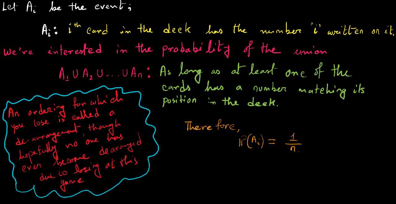
Consider a well-shuffled deck of \(n\) cards, labeled \(1\) through \(n\). You flip over the cards one by one, saying the numbers \(1\) through \(n\) as you do so. You win the game if, at some point, the number you say aloud is the same as the number on the card being flipped over (for example, if the \(7^{th}\) card in the deck has the label \(7\)). What is the probability of winning?

Mathematical Work

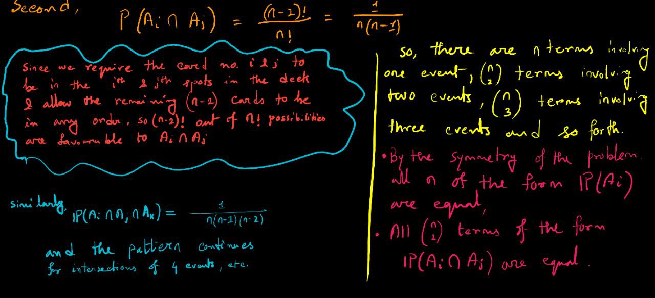
One way to see this is with the naive definition of probability, using the full sample space: there are \(n!\) possible orderings of the deck, all equally likely, and \((n−1)!\) of these are favorable to \(A_i\) (fix the card numbered \(i\) to be in the \(i^{th}\) position in the deck, and then the remaining \(n−1\) cards can be in any order). Another way to see this is by symmetry: the card numbered \(i\) is equally likely to be in any of the \(n\) positions in the deck, so it has probability \(1/n\) of being in the \(i^{th}\) spot.

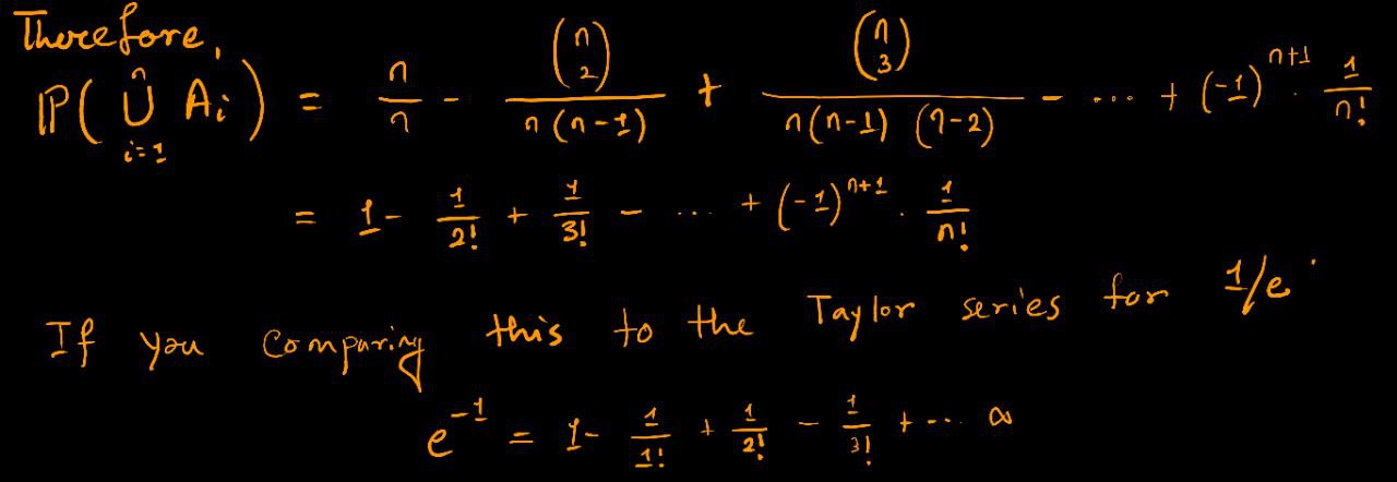
we see that for large \(n\), the probability of winning the game is extremely close to \(1 − 1/e\), or about \(0.63\). Interestingly, as \(n\) grows, the probability of winning approaches \(1 − 1/e\) instead of going to \(0\) or \(1\). With a lot of cards in the deck, the number of possible locations for matching cards increases while the probability of any particular match decreases, and these two forces offset each other and balance to give a probability of about \(1 − 1/e\).

R Programming Simulation

Let’s show by simulation that the probability of a matching card in this example is approximately \(1 − \frac{1}{e}\) when the deck is sufficiently large. Using R, we can perform the experiment a bunch of times and see how many times we encounter at least one matching card:

n <- 100
r <- replicate(10^4,sum(sample(n)==(1:n)))
sum(r>=1)/10^4

[1] 0.6367

In the first line, we choose how many cards are in the deck (here, 100 cards). In the second line, let’s work from the inside out:

• sample(n)==(1:n) is a vector of length \(n\), the \(i^{th}\) element of which equals \(1\) if the \(i^{th}\) card matches its position in the deck and \(0\) otherwise. That’s because for two numbers \(a\) and \(b\), the expression a==b is TRUE if a = b and FALSE otherwise, and TRUE is encoded as \(1\) and FALSE is encoded as 0.

• sum() adds up the elements of the vector, giving us the number of matching cards in this run of the experiment.

• replicate() does this \(10^4\) times. We store the results in r, a vector of length \(10^4\) containing the numbers of matched cards from each run of the experiment.

In the last line, we add up the number of times where there was at least one matching card, and we divide by the number of simulations.

To explain what the code is doing within the code rather than in separate documentation, we can add comments using the ’#’ symbol to mark the start of a comment. Comments are ignored by R but can make the code much easier to understand for the reader (who could be you—even if you will be the only one using your code, it is often hard to remember what everything means and how the code is supposed to work when looking at it a month after writing it). Short comments can be on the same line as the corresponding code; longer comments should be on separate lines. For example, a commented version of the above simulation is:

n <- 100       # number of cards
r <- replicate(10^4,sum(sample(n)==(1:n)))  # shuffle; count matches
sum(r>=1)/10^4    # proportion with a match

[1] 0.6319

We got \(0.637\), which is quite close to \(1 − \frac{1}{e}\).

Birthday Coincidences

There are \(k\) people in a room. Assume each person’s birthday is equally likely to be any of the \(365\) days of the year (we exclude February 29), and that people’s birthdays are independent (we assume there are no twins in the room). What is the probability that two or more people in the group have the same birthday?

Solution:

There are \(365^k\) ways to assign birthdays to the people in the room, since we can imagine the \(365\) days of the year being sampled \(k\) times, with replacement. By assumption, all of these possibilities are equally likely, so the naive definition of probability applies.

Used directly, the naive definition says we just need to count the number of ways to assign birthdays to k people such that there are two or more people who share a birthday. But this counting problem is hard, since it could be Fisher and Pearson who share a birthday, or Pearson and Rao, or all three of them, or the three of them could share a birthday while two others in the group share a different birthday, or various other possibilities.

Instead, let’s count the complement: the number of ways to assign birthdays to \(k\) people such that no two people share a birthday. This amounts to sampling the 365 days of the year without replacement, so the number of possibilities is \(365 · 364 · 363 · · · (365−k +1)\; \text{for}\; k \le 365\).

Therefore the probability of no birthday matches in a group of \(k\) people is

\[ P( \text{no birthday match }) = \dfrac{365 · 364 · 363 · · · (365−k +1)}{365^k} \]

and the probability of at least one birthday match is

\[ P ( \text{At least one birthday match}) = 1 - \dfrac{365 · 364 · 363 · · · (365−k +1)}{365^k} \]

Birthday Problem Calculation and Simulation

The following code uses prod() (which gives the product of a vector) to calculate the probability of at least one birthday match in a group of \(23\) people:

k <- 23
1-prod((365-k+1):365)/365^k

[1] 0.5072972

Better yet, R has built-in functions, pbirthday() and qbirthday(), for the birthday problem! pbirthday(k) returns the probability of at least one match if the room has \(k\) people. qbirthday(p) returns the number of people needed in order to have probability \(p\) of at least one match. For example,

pbirthday(23)

[1] 0.5072972

qbirthday(0.5)

[1] 23

We can also find the probability of having at least one triple birthday match, i.e., three people with the same birthday; all we have to do is add coincident=3 to say we’re looking for triple matches. For example,

pbirthday(23,coincident=3)

[1] 0.01441541

So \(23\) people give us only a 1.4% chance of a triple birthday match.

qbirthday(0.5,coincident=3) 

[1] 88

so we’d need \(88\) people to have at least a 50% chance of at least one triple birthday match. To simulate the birthday problem, we can use

b <- sample(1:365,23,replace=TRUE)
tabulate(b)

  [1] 0 1 0 0 0 0 0 0 0 0 1 0 0 0 0 0 0 0 0 0 0 0 0 0 0 0 0 0 0 0 0 0 0 0 0 0 0
 [38] 0 0 0 0 0 0 1 0 0 0 0 0 0 0 0 0 0 0 0 0 0 0 0 0 0 0 0 0 0 0 0 0 0 0 0 0 0
 [75] 0 0 0 0 0 0 0 0 0 0 0 0 0 0 1 0 0 0 0 1 0 0 0 1 1 0 0 0 0 0 0 0 0 0 0 0 0
[112] 0 0 0 0 0 0 0 0 0 0 0 0 0 0 0 0 0 0 0 0 0 0 0 0 1 0 0 0 0 0 0 0 0 0 0 0 0
[149] 0 0 0 0 0 0 0 0 0 0 0 0 0 0 1 0 0 0 0 0 0 0 0 0 1 0 0 0 0 0 0 0 0 0 0 0 0
[186] 0 0 0 1 0 0 0 0 0 0 0 1 0 0 0 0 0 0 0 0 0 0 0 0 0 0 0 0 0 0 0 0 0 0 0 0 1
[223] 0 0 0 0 0 0 0 0 0 0 0 0 1 0 0 0 1 0 0 0 0 0 0 0 1 0 0 0 0 0 0 0 1 0 0 0 0
[260] 0 0 0 0 0 0 0 0 0 0 0 0 0 0 0 0 0 0 0 0 0 0 0 0 0 0 0 0 0 0 0 1 0 0 0 0 0
[297] 0 0 0 0 0 0 0 1 0 0 0 0 0 0 0 0 0 0 0 0 0 0 0 0 0 1 0 0 0 0 0 0 0 0 0 1 0
[334] 0 0 0 0 0 0 0 0 0 0 0 0 0 0 0 0 0 0 0 0 0 0 1 0 0 0 0 0 0 0 1

to generate random birthdays for \(23\) people and then tabulate the counts of how many people were born on each day (the command tabulate(b) creates a prettier table, but is slower). We can run \(10^4\) repetitions as follows:

r <- replicate(10^4, max(tabulate(sample(1:365,23,replace=TRUE))))
sum(r>=2)/10^4

[1] 0.508

If the probabilities of various days are not all equal, the calculation becomes much more difficult, but the simulation can easily be extended since sample allows us to specify the probability of each day (by default sample assigns equal probabilities, so in the above the probability is \(\frac{1}{365}\) for each day).

Different Approach & Visualization

If there are \(23\) individuals in a room, there is a \(50-50\) chance two individuals will have the same birthday

k = 23  # number of people in room
p <- numeric(k)  # create numeric vector to store probabilities
for (i in 1:k)      {
            q <- 1 - (0:(i - 1))/365  # 1 - prob(no matches)
            p[i] <- 1 - prod(q)  }
prob <- p[k]
prob

[1] 0.5072972

Generalized probability that at least \(2\) individuals will have same birthday in a room of \(k\) people

k = 100  # number of people in room
p <- numeric(k)  # create numeric vector to store probabilities
for (i in 1:k)      {
            q <- 1 - (0:(i - 1))/365  # 1 - prob(no matches)
            p[i] <- 1 - prod(q)  }
plot(p, main="Probability at least 2 people have same Birthday", 
        xlab ="Number of People", 
        ylab = "Probability", col="blue")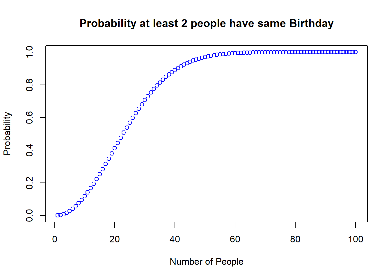        

The probability of two individuals having the same birthday quickly increases:

• 50% probability if 23 people in the room

• Over 80% probability if 35 people in the room

• Over 99% probability if 57 people in the room

Number.of.People <-c(seq(1,100,1))
Probabilities <- format(p, digits=3)
probs <- cbind(Number.of.People, Probabilities )   
#Output Table
DT::datatable(probs, rownames=FALSE,
              options = list(autowidth=TRUE,
              sClass="alignCenter",
              className = 'dt-Center',
              pageLength=10))

Random Committees

Q1. In the U.S. Senate, a committee of \(50\) senators is chosen at random. What is the probability that Massachusetts is represented? What is the probability that every state is represented?

In any real committee the members are not chosen at random. What this question is implicitly asking is whether random choice is “reasonable” with respect to two criteria of reasonableness. Note that the phrase “at random” is ambiguous. A more precise statement would be that every \(50\) senator committee is as probable as any other.

We first count \(|\Omega|\), the number of possible committees. Since \(50\) senators are being chosen from \(100\) senators, there are

\[ |\Omega| = \binom{100}{50} \]

committees. Let \(A\) be the event “Massachusetts is not represented.” The committees in \(A\) consist of \(50\) senators chosen from the \(98\) non-Massachusetts senators. Therefore,

\[ |A| = \binom{98}{50} \]

The probability of \(A\) is easily evaluated by using the R function choose that computes the binomial coefficient:

choose(98,50)/choose(100,50)

[1] 0.2474747

So the answer to our original question is that Massachusetts is represented with probability \(1 − 0.247 = 0.753\) or \(3\) to \(1\) odds. This seems reasonable. Now consider the event \(A\) = “Every state is represented.” Each committee in \(A\) is formed by making \(50\) independent choices from the \(50\) state delegations. Hence \(|A| = 250\) and the probability is

2^50/choose(100,50)

[1] 1.115953e-14

This probability is so small that the event \(A\) is essentially impossible. By this criterion, random choice is not a reasonable way to choose a committee. Some binomial coefficients are so large that choose will cause the computation to fail. In such a case, one should use the lchoose() function, which computes the logarithm of the binomial coefficient.

Q2. Some environmentalists want to estimate the number of whitefish in a small lake. They do this as follows. First \(50\) whitefish are caught, tagged and returned to the lake. Some time later another \(50\) are caught and they find \(3\) tagged ones. For each n compute the probability that this could happen if there are n whitefish in the lake. For which n is this probability the highest? Is this a reasonable estimate for \(n\)?

After tagging, there are \(50\) tagged fish and \((n − 50)\) untagged ones. Catching \(50\) fish can be done in \(\binom{n}{50}\) ways, while one can catch \(3\) tagged and \(47\) untagged fish in \(\binom{50}{3} . \binom{n-50}{47}\) ways. So if this event is written \(A_n\), then we can write the probability of this event in R as follows:

n <- 50 : 2000
fish <- function(n){
  choose(50,3)*choose(n-50,47)/choose(n,50)
}
plot(n,fish(n),type = "l")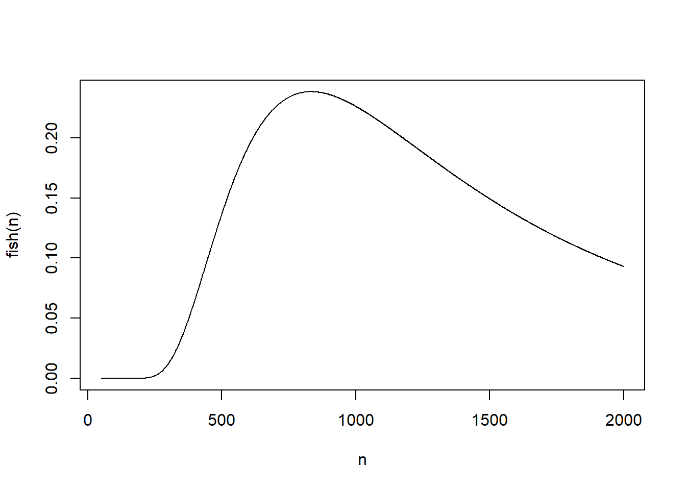

So far all of our graphs have been simple point plots. This time, instead of drawing points, we want to draw a curve. In R, this is called a “line graph,” and it is specified by using the type="l" parameter. Here is a line graph of our fish function from \(50\) to \(2000\)

The maximum is easily computed to be max(fish(n)). Finding where this maximum occurs is easily done by selecting the components of the vector \(n\) where the maximum occurs. This will, in general, select all of the values of the vector \(n\) where the maximum occurs, but in this case it occurs just once:

m <- max(fish(n))
m

[1] 0.2382917

n[fish(n)==m]

[1] 833

Notice that while \(n = 833\) is the value of n that maximizes \(P(A_n)\), it is only slightly better than neighboring values. For example, fish(830) = 0.238287. Indeed, \(A_n\) is not a very likely event for any \(n\) in the interval from \(450\) to \(1900\). It is never higher than 24%. We will discuss this problem in the context of statistical hypothesis testing.

Exercise

1. A group of astrologers has, in the past few years, cast some \(20,000\) horoscopes. Consider only the positions (houses) of the sun, the moon, Mercury, Venus, Earth, Mars, Jupiter and Saturn. There are \(12\) houses in the Zodiac. Assuming complete randomness, what is the probability that at least \(2\) of the horoscopes were the same?

2. It is an old Chinese custom to play a dice game in which six dice are rolled and prizes are awarded according to the pattern of the faces shown, ranging from “all faces the same” (highest prize) to “all faces different.” List the possible patterns obtainable and compute the probabilities. Do you notice any surprises?