The Classical Approach For Probability
Introduction
The mathematical foundation of probability is rooted in the concept of sets. Consider an experiment where a set of potential outcomes exists. Before experimenting, the specific outcome remains unknown, and the possibilities are encapsulated within the set. For instance, envision tossing a coin—a simple experiment with two potential outcomes: heads or tails. Before the coin is tossed, the set of possibilities is {Heads, Tails}. This set represents all conceivable outcomes. The actual act of tossing the coin constitutes the experiment. While the coin is in mid-air, any outcome from the set could materialize. It is only after the coin lands that the uncertainty surrounding the outcome is resolved. The result then “crystallizes” into the actual outcome, whether it be Heads or Tails. In the language of sets and probability, the set {Heads, Tails} embodies all conceivable outcomes, and the probability associated with each outcome before the toss is \(1/2\) (assuming a fair coin). Following the toss, the probability of the realized outcome becomes 1, signifying that the uncertainty has transformed into a definite outcome. This illustrates the core idea that probability provides a means of quantifying uncertainty, marking the transition from a set of potential outcomes to the actualized outcome after the experiment.
Sample spaces and Pebble World
Sample Space
In probability theory, a sample space is a fundamental concept representing the set of all possible outcomes of a particular experiment. It serves as the universe from which we draw potential results. Consider rolling a six-sided die; the sample space for this experiment would be {1, 2, 3, 4, 5, 6}, as these are all the possible outcomes.
Diving into Pebble World
Now, let’s introduce the concept of the Pebble World as a metaphorical tool to understand probability. Imagine placing pebbles on different points within the sample space, where each pebble corresponds to a possible outcome. The density or number of pebbles on a specific outcome reflects the likelihood or probability of that outcome occurring. For instance, let’s return to the six-sided die. If the die is fair, each number from \(1\) to \(6\) has an equal chance of occurring. In the Pebble World, this would mean placing an equal number of pebbles on each corresponding point in the sample space. However, if the die is biased, favoring certain numbers over others, more pebbles would be placed on those specific points in the sample space. The distribution of pebbles illustrates the probability distribution of outcomes, providing a visual representation of the likelihood of each result. The Pebble World concept aids in grasping the fundamental idea that the sample space encompasses all conceivable outcomes, and the arrangement of pebbles within it signifies the probabilities associated with each outcome. It offers an intuitive way to visualize and understand the probabilistic nature of random experiments, making complex probability concepts more accessible and tangible.
Definition(Sample space and event): The sample space \(S\) of an experiment is the set of all possible outcomes of the experiment. An event \(A\) is a subset of the sample space \(S\), and we say that \(A\) occurred if the actual outcome is in \(A\).
The sample space of an experiment can be finite, countably infinite, or uncountably infinite.
Justification of Countable & Uncountable Sets
Mathematics Behind the Concept
A set may be finite or infinite. If \(A\) is a finite set, we write \(|A|\) for the number of elements in \(A\), which is called its size or cardinality. For example, \(| \{2, 4, 6, 8, 10\}| = 5\) since there are \(5\) elements in this set. A very useful fact is that \(A\) and \(B\) are finite sets, then
\[ | A\cup B| = |A| +|B| - |A\cap B| \]
This is a form of the inclusion-exclusion. It says that to count how many elements are in the union of \(A\) and \(B\), we can add the separate counts for each, and then adjust for the fact that we have double-counted the elements (if any) that are in both \(A\) and \(B\). Two sets \(A\) and \(B\) are said to have the same size or same cardinality if they can be put into one-to-one correspondence, i.e., if each element of \(A\) can be paired up with exactly one element of \(B\), with no unpaired elements in either set. We say that \(A\) is smaller than \(B\) if there is not a one-to-one correspondence between \(A\) and \(B\), but there is a one-to-one correspondence between \(A\) and a subset of \(B\).
Example
For example, suppose that we want to count the number of people in a movie theater with \(100\) seats. Assume that no one in the theater is standing, and no seat has more than one person in it. The obvious thing to do is to go around counting people one by one (though it’s surprisingly easy to miss someone or accidentally count someone twice). But if every seat is occupied, then a much easier method is to note that there must be \(100\) people, since there are \(100\) seats and there is a one-to-one correspondence between people and seats. If some seats are empty, then there must be fewer than \(100\) people there.
Paradoxical Justification
This idea of looking at one-to-one correspondences makes sense both for finite and infinite sets. Consider the perfect squares \(1^2, 2^2, 3^2, . . .\) . Galileo pointed out the paradoxical result that on the one hand it seems like there are fewer perfect squares than positive integers (since every perfect square is a positive integer, but lots of positive integers aren’t perfect squares), but on the other hand it seems like these two sets have the same size since they can be put into one-to-one correspondence: pair \(1^2\) with \(1\), pair \(2^2\) with \(2\), pair \(3^2\) with \(3\), etc. Galileo’s paradox resolves to realize that intuitions about finite sets don’t necessarily carry over to infinite sets. By definition, the set of all perfect squares and the set of all positive integers do have the same size.
Hilbert’s Infinite Hotel Paradox
Another famous example of this is Hilbert’s hotel. For any hotel in the real world, the number of rooms is finite. If every room is occupied, there is no way to accommodate more guests, other than by cramming more people into already occupied rooms. Now consider an imaginary hotel with an infinite sequence of rooms, numbered \(1, 2, 3, . . .\) . Assume that all the rooms are occupied and that a weary traveler arrives, looking for a room.
Can the hotel give the traveler a room, without leaving any of the current guests without a room?
Yes, one way is to have the guest in room \(n\) move to room \(n+1\), for all \(n = 1, 2, 3,\ldots\). This frees up room \(1\), so the traveler can stay there.
What if infinitely many travelers arrive at the same time, such that their cardinality is the same as that of the positive integers (so we can label the travelers as traveler 1, traveler 2, . . . )?
The hotel could fit them in one by one by repeating the above procedure over and over again, but it would take forever (infinitely many moves) to accommodate everyone, and it would be bad for business to make the current guests keep moving over and over again.
Can the room assignments be updated just once so that everyone has a room?
Yes, one way is to have the guest in room n move to room to \(2n\) for all \(n = 1, 2, 3, \ldots\) , and then have traveler n move into room \(2n − 1\). In this way, the current guests occupy all the even-numbered rooms, and the new guests occupy all the odd-numbered rooms.
An infinite set is called countably infinite if it has the same cardinality as the set of all positive integers. A set is called countable if it is finite or countably infinite, and uncountable otherwise. The mathematician Cantor showed that not all infinite sets are the same size. In particular, the set of all real numbers is uncountable, as is any interval in the real line of positive length.
Numerical Problems
Experimenting amounts to randomly selecting one pebble. If all the pebbles are of the same mass, all the pebbles are equally likely to be chosen. This special case is the topic of our upcoming sessions. Set theory is very useful in probability since it provides a rich language for expressing and working with events. Set operations, especially unions, intersections, and complements, make it easy to build new events in terms of already-defined events. These concepts also let us express an event in more than one way; often, one expression for an event is much easier to work with than another expression for the same event.
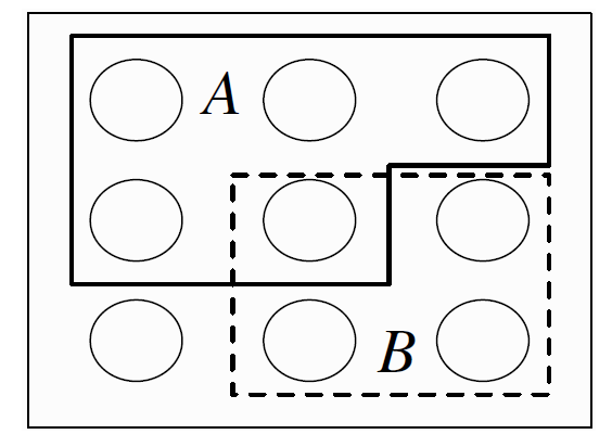
For example, let \(S\) be the sample space of an experiment and let \(A,B \subseteq S\) be events. Then the union \(A \cup B\) is the event that occurs iff at least one of \(A\) and \(B\) occurs, the intersection \(A \cap B\) is the event that occurs if and only if both \(A\) and \(B\) occur, and the complement \(A^c\) is the event that occurs iff \(A\) does not occur. We also have De Morgan’s laws:
\[ (A\cup B)^c = A^c \cap B^c \; and\;(A\cap B)^c =A^c \cup B^c \]
since saying that it is not the case that at least one of \(A\) and \(B\) occur is the same as saying that \(A\) does not occur and \(B\) does not occur, and saying that it is not the case that both occur is the same as saying that at least one does not occur. Analogous results hold for unions and intersections of more than two events. In the example shown in Fig 1.1, \(A\) is a set of \(5\) pebbles, \(B\) is a set of \(4\) pebbles, \(A \cup B\) consists of the \(8\) pebbles in \(A\) or \(B\) (including the pebble that is in both), \(A \cap B\) consists of the pebble that is in both \(A\) and \(B\), and \(A^c\) consists of the \(4\) pebbles that are not in \(A\).
The notion of sample space is very general and abstract, so it is important to have some concrete examples in mind.
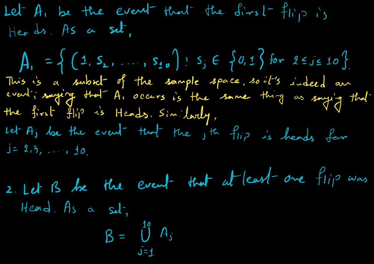
Coin Flip Example
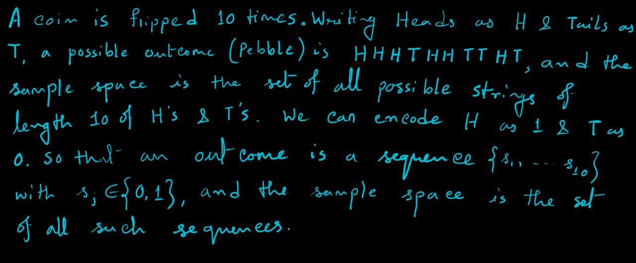
.jpg)
(Pick a Card, Any Card) Example
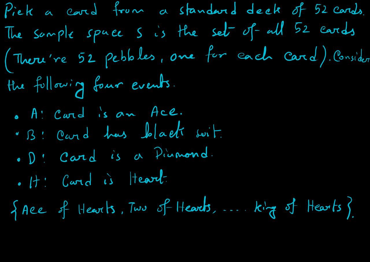
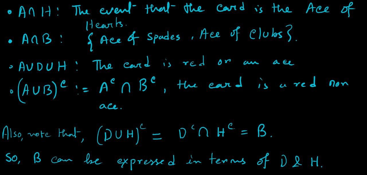
On the other hand, the event that the card is a spade can’t be written in terms of \(A,B,D,H\) since none of them are fine-grained enough to be able to distinguish between spades and clubs.
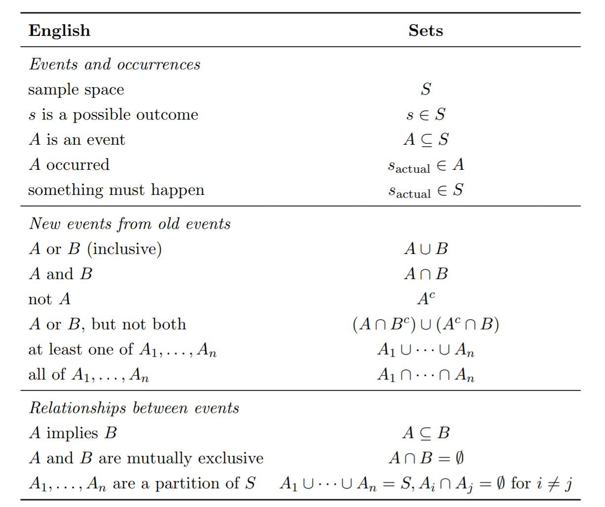
Convertion Between English and Sets
As the preceding examples demonstrate, events can be described in English or set notation. Sometimes the English description is easier to interpret while the set notation is easier to manipulate. Let \(S\) be a sample space and \(s_{actual}\) be the actual outcome of the experiment (the pebble that ends up getting chosen when the experiment is performed). A mini-dictionary for converting between English and sets is given below.
Naive Definition of Probability
Historically, the earliest definition of the probability of an event was to count the number of ways the event could happen and divide by the total number of possible outcomes for the experiment. We call this the naive definition since it is restrictive and relies on strong assumptions; nevertheless, it is important to understand, and useful when not misused.
Definition:
Naive definition of probability: Let \(A\) be an event for an experiment with a finite sample space \(S\). The naive probability of \(A\) is
\[ P _{Naive}(A) = \dfrac{|A|}{|S|} = \dfrac{\text{No. of outcomes favourable in A}}{{\text{Total number of outcomes in S}}} \]
\(|A|\) to denote the size of \(A\);
In terms of Pebble World, the naive definition just says that the probability of \(A\) is the fraction of pebbles that are in \(A\). For example, in figure it says,
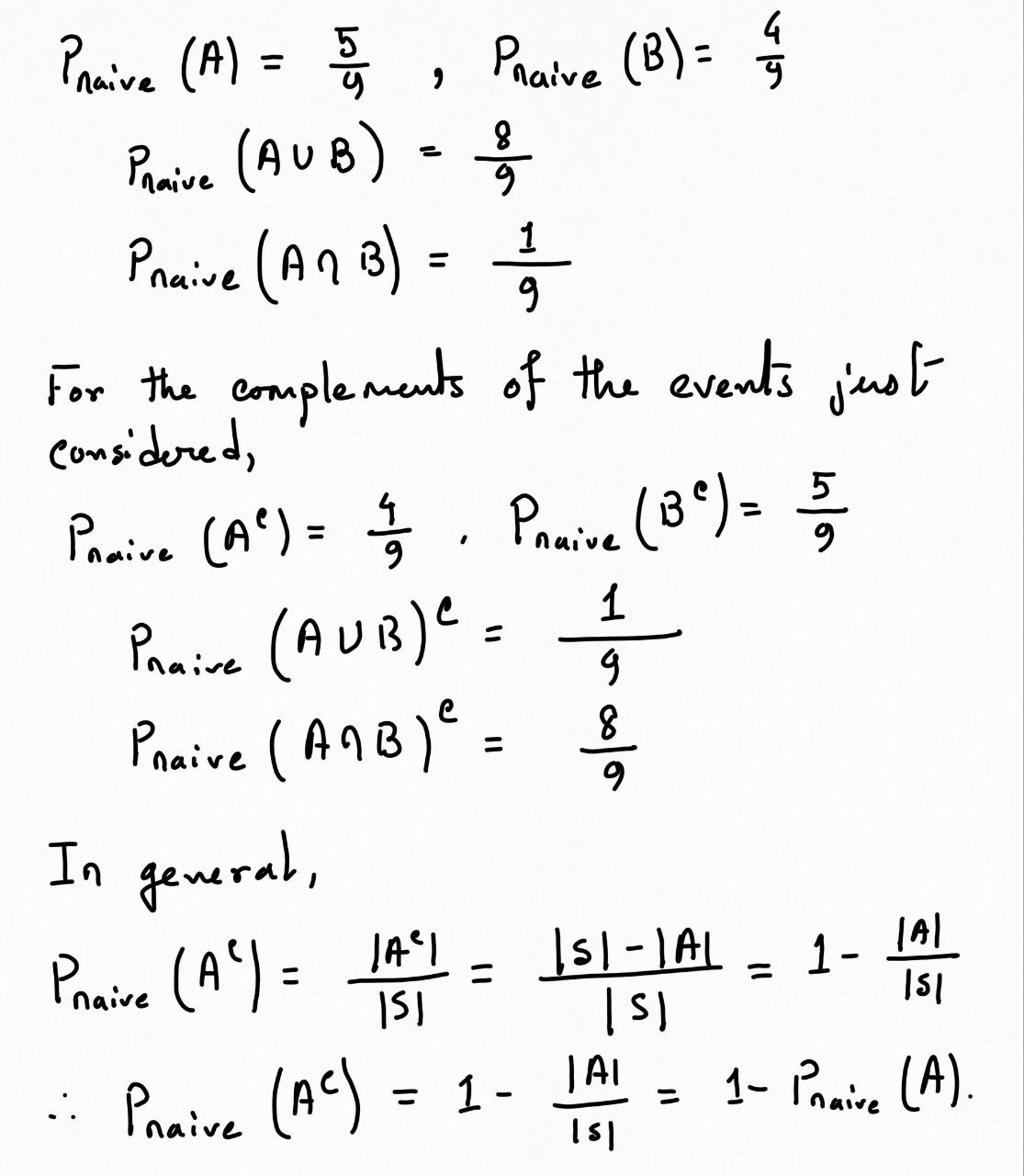
A good strategy when trying to find the probability of an event is to start by thinking about whether it will be easier to find the probability of the event or the probability of its complement. The naive definition is very restrictive in that it requires \(S\) to be finite, with equal mass for each pebble. It has often been misapplied by people who assume equally likely outcomes without justification and make arguments to the effect of “either it will happen or it won’t, and we do not know which, so it’s \(50-50\)”.
In addition to sometimes giving absurd probabilities, this type of reasoning isn’t even internally consistent. For example, it would say that the probability of life on Mars is \(1/2\) (“either there is or there isn’t life there”), but it would also say that the probability of intelligent life on Mars is \(1/2\), and it is clear intuitively—and by the properties of probability developed in upcoming session —that the latter should have a strictly lower probability than the former. But there are several important types of problems where the naive definition is applicable:
when there is symmetry in the problem that makes outcomes equally likely. It is common to assume that a coin has a 50% chance of landing Heads when tossed, due to the physical symmetry of the coin. For a standard, well-shuffled deck of cards, it is reasonable to assume that all orders are equally likely. There aren’t certain overeager cards that especially like to be near the top of the deck; any particular location in the deck is equally likely to house any of the \(52\) cards.
when the outcomes are equally likely by design. For example, consider conducting a survey of \(n\) people in a population of \(N\) people. A common goal is to obtain a simple random sample, which means that the n people are chosen randomly with all subsets of size \(n\) being equally likely. If successful, this ensures that the naive definition is applicable, but in practice, this may be hard to accomplish because of various complications, such as not having a complete, accurate list of contact information for everyone in the population.
when the naive definition serves as a useful null model. In this setting, we assume that the naive definition applies just to see what predictions it would yield, and then we can compare observed data with predicted values to assess whether the hypothesis of equally likely outcomes is tenable.
Remarks:
See Diaconis, Holmes, and Montgomery [1]for a physical argument that the chance of a tossed coin coming up the way it started is about \(0.51\) (close to but slightly more than \(1/2\)), and Gelman and Nolan [2]for an explanation of why the probability of Heads is close to \(1/2\) even for a coin that is manufactured to have different weights on the two sides (for standard coin-tossing; allowing the coin to spin is a different matter).
Lecture Videos
See Also
References
Persi Diaconis. The Markov chain Monte Carlo revolution. Bulletin of the American Mathematical Society, 46(2):179–205, 2009.
Andrew Gelman, John B. Carlin, Hal S. Stern, David B. Dunson, Aki Vehtari, and Donald B. Rubin. Bayesian Data Analysis. CRC Press, 2013.