“In the intricate patterns of fractal canopies, we glimpse the artistry of mathematics and the poetry of nature.”
Canopy Chronicles
Picture yourself standing in a lush, dense forest, surrounded by towering canopy trees reaching towards the sky. As you gaze upward, you’re mesmerized by the intricate patterns and branching structures, reminiscent of a fractal canopy unfolding above you. The canopy of a forest is like a vast green umbrella, providing shelter and habitat for countless organisms below. Similarly, the fractal nature of the canopy mimics the self-similar patterns found in fractals, where each branch and leaf is a miniature reflection of the whole. Just as a single canopy tree can be seen as a microcosm of the entire forest ecosystem, with its micro-habitats and inhabitants, a fractal canopy exhibits a similar principle on a visual scale. Zoom in on any part of the canopy, and you’ll find the same repeating patterns branching out infinitely, like a natural work of art crafted by the laws of mathematics and growth.
Canopy of a Forest
Canopy Layers
From Doodling to Natural Phenomena
Imagine you’re doodling with a pencil on a piece of paper, drawing a simple line. Now, imagine you decide to get a bit fancier and split that line into two smaller lines at the end. Next, you decide to do the same thing to each of those smaller lines, splitting them into even smaller lines. You keep doing this over and over again, each time splitting the lines into smaller and smaller pieces.
That’s essentially how a fractal canopy forms. It starts with a simple line, and then it gets split and branched into smaller lines sequentially. At the end of each line, new lines are drawn at specific angles, creating a branching pattern that keeps repeating. Now, here’s where it gets interesting. There are a bunch of things you can tweak to change how the fractal canopy looks. You can play around with the number of branches, deciding how many lines to split each existing line into. You can also adjust the angle between the branches, determining how they spread out from each other. And don’t forget about the original width of the lines and how that changes as the branches get smaller. It’s like having a whole toolbox of options to create different kinds of fractal canopies.
At the heart of fractal canopy generation lies the interplay of fundamental parameters: the number of branches, the angle of divergence, and the decay of length and width. These parameters serve as the building blocks of creativity, allowing you to sculpt the canopy’s form and texture with precision and finesse. By manipulating these variables, you can sculpt a symphony of shapes ranging from graceful arches to intricate networks, each bearing the hallmark of your artistic vision. But the allure of fractal canopies extends far beyond the realm of aesthetics. Embedded within their intricate patterns lie profound insights into the principles of growth and organization that govern natural phenomena. Take, for instance, the branching structures of trees and plants, which mirror the recursive branching of fractal canopies. By studying these natural analogs, scientists gain invaluable insights into the optimization of resource distribution and the resilience of ecosystems.
Nature’s Fractal Symphony: The Beauty of Recursive Growth
In nature, both trees and forest canopies follow similar rules to grow. It’s like when you see a big tree in the woods, and then you notice that its smaller branches look just like the big ones. This happens again and again, making the whole forest look like a big version of one small part. It’s like nature’s way of using the same pattern over and over to create something big and beautiful. Understanding how trees grow like this helps us see how nature works in a simple but cool way.
Recursive trees, a fundamental concept in computing and mathematics, illustrate the idea of self-similarity and iteration. Starting with a single trunk, they grow into larger branches, which then split into smaller branches recursively. This process repeats indefinitely, creating increasingly complex patterns. Despite their complexity, recursive trees are easy to understand at first glance. Watching the initial stages reveals the concept. They demonstrate how simplicity leads to complexity through repetition. Recursive trees show nature’s algorithm, where each step builds on the last, resulting in orderly growth. In summary, they highlight the power of recursion in creating complex structures from simple elements.
Investigation into Iterative Drawing Algorithms
In this article, we’re investigating the implementation and application of iterative drawing algorithms, particularly focusing on recursive tree generation. The primary objective is to explore the rationale behind the development of code segments aimed at creating intricate tree-like structures through iterative processes.
1.1 Code
Code
# function to draw a single linedrawLine <-function(line, col="white", lwd=1) {segments(x0=line[1], y0=line[2], x1=line[3], y1=line[4], col=col,lwd=lwd)}# wrapper around "drawLine" to draw entire objectsdrawObject <-function(object, col="white", lwd=1) {invisible(apply(object, 1, drawLine, col=col, lwd=lwd))}# exampleline1 =c(0,0,1,1)line2 =c(-3,4,-2,-4)line3 =c(1,-3,4,3)mat =matrix(c(line1,line2,line3), byrow=T, nrow=3)# function to add a new line to an existing onenewLine <-function(line, angle, reduce=1) { x0 <- line[1] y0 <- line[2] x1 <- line[3] y1 <- line[4] dx <-unname(x1-x0) # change in x direction dy <-unname(y1-y0) # change in y direction l <-sqrt(dx^2+ dy^2) # length of the line theta <-atan(dy/dx) *180/ pi # angle between line and origin rad <- (angle+theta) * pi /180# (theta + new angle) in radians coeff <-sign(theta)*sign(dy) # coefficient of directionif(coeff ==0) coeff <--1 x2 <- x0 + coeff*l*cos(rad)*reduce + dx # new x location y2 <- y0 + coeff*l*sin(rad)*reduce + dy # new y locationreturn(c(x1,y1,x2,y2))}# function to run next iteration based on "ifun()"iterate <-function(object, ifun, ...) { linesList <-vector("list",0)for(i in1:nrow(object)) { old_line <-matrix(object[i,], nrow=1) new_line <-ifun(old_line, ...) linesList[[length(linesList)+1]] <- new_line } new_object <-do.call(rbind, linesList)return(new_object)}# iterator function: recursive treetree <-function(line0, angle=30, reduce=.7, randomness=0) {# angles and randomness angle1 <- angle+rnorm(1,0,randomness) # left branch angle2 <--angle+rnorm(1,0,randomness) # right branch# new branches line1 <-newLine(line0, angle=angle1, reduce=reduce) line2 <-newLine(line0, angle=angle2, reduce=reduce)# store in matrix and return mat <-matrix(c(line1,line2), byrow=T, ncol=4)return(mat)}
1.1 Interpretation
The article helps us explore a function for adding new lines based on specified angles, facilitating the iterative expansion of geometric structures. Central to the investigation is the iterate and tree functions, which enable recursive tree generation by iteratively applying transformations to construct branching patterns. Through a blend of mathematical computation and algorithmic logic, these functions facilitate the creation of visually captivating patterns with applications in computer graphics and computational art. Understanding the principles behind these algorithms offers opportunities for further exploration and extension in iterative drawing techniques.
1.2 Code
Code
# function to create empty canvasemptyCanvas <-function(xlim, ylim, bg="gray20") {par(mar=rep(1,4), bg=bg)plot(1, type="n", bty="n",xlab="", ylab="", xaxt="n", yaxt="n",xlim=xlim, ylim=ylim)}# exampleemptyCanvas(xlim=c(0,1), ylim=c(0,1))# example: recursive tree (First iterations)fractal <-matrix(c(0,0,0,10), nrow=1)emptyCanvas(xlim=c(-30,30), ylim=c(0,35))drawObject(fractal)for(i in1:1) { fractal <-iterate(fractal, ifun=tree, angle=23)drawObject(fractal)}# example: recursive tree (after two iterations)fractal <-matrix(c(0,0,0,10), nrow=1)emptyCanvas(xlim=c(-30,30), ylim=c(0,35))drawObject(fractal)for(i in1:2) { fractal <-iterate(fractal, ifun=tree, angle=23)drawObject(fractal)}# example: recursive tree (after three iterations)fractal <-matrix(c(0,0,0,10), nrow=1)emptyCanvas(xlim=c(-30,30), ylim=c(0,35))drawObject(fractal)for(i in1:3) { fractal <-iterate(fractal, ifun=tree, angle=23)drawObject(fractal)}# example: recursive tree (after four iterations)fractal <-matrix(c(0,0,0,10), nrow=1)emptyCanvas(xlim=c(-30,30), ylim=c(0,35))drawObject(fractal)for(i in1:4) { fractal <-iterate(fractal, ifun=tree, angle=23)drawObject(fractal)}# example: recursive tree (after six iterations)fractal <-matrix(c(0,0,0,10), nrow=1)emptyCanvas(xlim=c(-30,30), ylim=c(0,35))drawObject(fractal)for(i in1:6) { fractal <-iterate(fractal, ifun=tree, angle=23)drawObject(fractal)}
1.2 Interpretation
Above code defines a function emptyCanvas that creates an empty plot with specified x and y limits, and a background color. The function is then called with different parameters to create empty canvases for subsequent plots. After defining the emptyCanvas function, the code proceeds to generate examples of recursive trees using a custom function tree and two helper functions iterate and drawObject. Each example demonstrates the recursive tree at different stages of iteration.
For each example:
The fractal matrix is initialized with starting coordinates.
An empty canvas is created using emptyCanvas with specified x and y limits.
The initial object represented by fractal is drawn using drawObject.
A for loop iterates over a specified number of iterations (1, 2, 3, 4, and 6 in different examples).
In each iteration, the fractal matrix is updated using the iterate function with a specified angle.
The updated fractal object is drawn using drawObject.
These examples illustrate how recursive trees grow and become more complex with each iteration, demonstrating the power of recursion in generating intricate patterns.
1.3 Code
Code
# iterator function: recursive tree(After 10 iteration )tree <-function(line0, angle=30, reduce=.7, randomness=0) {# angles and randomness angle1 <- angle+rnorm(1,0,randomness) # left branch angle2 <--angle+rnorm(1,0,randomness) # right branch# new branches line1 <-newLine(line0, angle=angle1, reduce=reduce) line2 <-newLine(line0, angle=angle2, reduce=reduce)# store in matrix and return mat <-matrix(c(line1,line2), byrow=T, ncol=4)return(mat)}# example: recursive tree (after ten iterations)fractal <-matrix(c(0,0,0,10), nrow=1)emptyCanvas(xlim=c(-30,30), ylim=c(0,35))drawObject(fractal)for(i in1:10) { fractal <-iterate(fractal, ifun=tree, angle=23)drawObject(fractal)}
1.3 interpretation
This code visually demonstrates the growth of a recursive tree after ten iterations, showcasing how the tree branches out and becomes more complex with each iteration. The tree function defines the process of creating new branches for the recursive tree. Here’s a breakdown of how it works:
Inputs: It takes a line segment (line0) representing the current branch, along with optional parameters such as the angle of rotation (angle), reduction factor (reduce), and randomness (randomness).
Branch Angles: It calculates two new angles (angle1 and angle2) by adding and subtracting a random value from the specified angle. This introduces randomness to the branching angles, making the tree appear more natural.
New Branches: It creates two new line segments (line1 and line2) based on the original line segment and the calculated angles. These represent the left and right branches of the current branch.
Output: It stores the coordinates of the new line segments in a matrix (mat) and returns it.
After defining the tree function, the code proceeds to visualize the recursive tree after ten iterations. Here’s what happens:
An initial line segment (fractal) is defined as a matrix with coordinates (0,0,0,10), representing the trunk of the tree.
An empty canvas is created with specified x and y limits using the emptyCanvas function (not shown in this code snippet).
The initial line segment (fractal) is drawn on the canvas using the drawObject function.
A for loop iterates ten times, each time applying the tree function to the current line segment (fractal) to generate new branches. The angle of rotation is set to 23 degrees for each iteration.
After each iteration, the updated line segment (fractal) is drawn on the canvas using the drawObject function.
1.4 Code
Code
# example: recursive tree (after 10 iterations with colors)fractal <-matrix(c(0,0,0,10), nrow=1)emptyCanvas(xlim=c(-30,30), ylim=c(0,35))drawObject(fractal)for(i in1:10) { fractal <-iterate(fractal, ifun=tree, angle=23)drawObject(fractal,col=i+1)}# example: recursive tree (after 12 iterations with colors)fractal <-matrix(c(0,0,0,10), nrow=1)emptyCanvas(xlim=c(-30,30), ylim=c(0,35))drawObject(fractal)for(i in1:12) { fractal <-iterate(fractal, ifun=tree, angle=23)drawObject(fractal,col=i+1)}# example: recursive tree (after 14 iterations with colors)fractal <-matrix(c(0,0,0,10), nrow=1)emptyCanvas(xlim=c(-30,30), ylim=c(0,35))drawObject(fractal)for(i in1:14) { fractal <-iterate(fractal, ifun=tree, angle=23)drawObject(fractal,col=i+1)}# example: recursive tree (after 16 iterations with colors)fractal <-matrix(c(0,0,0,10), nrow=1)emptyCanvas(xlim=c(-30,30), ylim=c(0,35))drawObject(fractal)for(i in1:16) { fractal <-iterate(fractal, ifun=tree, angle=23)drawObject(fractal,col=i+1)}# example: recursive tree (after 18 iterations with colors)fractal <-matrix(c(0,0,0,10), nrow=1)emptyCanvas(xlim=c(-30,30), ylim=c(0,35))drawObject(fractal)for(i in1:18) { fractal <-iterate(fractal, ifun=tree, angle=23)drawObject(fractal,col=i+1)}# example: recursive tree (after 20 iterations with colors)fractal <-matrix(c(0,0,0,10), nrow=1)emptyCanvas(xlim=c(-30,30), ylim=c(0,35))drawObject(fractal)for(i in1:20) { fractal <-iterate(fractal, ifun=tree, angle=23)drawObject(fractal,col=i+1)}
1.4 Interpretation
This code generates and visualizes recursive trees with varying complexity, showing the growth and branching patterns over multiple iterations. The use of different colors for each iteration enhances the visualization and makes it easier to observe the progression of tree growth. This code illustrates the generation of recursive trees with different numbers of iterations, each represented with a distinct color for visual distinction.
Setting up the canvas:
A starting line segment (fractal) is defined as a matrix representing the trunk of the tree.
An empty canvas with specified x and y limits is created using the emptyCanvas function.
Drawing the initial tree trunk:
The starting line segment (fractal) is drawn on the canvas using the drawObject function.
Iterating over the tree growth:
A for loop iterates over a range of iterations (10, 12, 14, 16, 18, and 20).
In each iteration, the tree function is applied to the current line segment (fractal) to generate new branches.
The angle of rotation is set to 23 degrees for each iteration.
The iterate function updates the line segments based on the tree function.
The updated line segments are drawn on the canvas using the drawObject function, with each iteration represented by a different color (col=i+1).
These sections of code generate organic recursive trees with a tapered appearance and visualize their growth over multiple iterations. The use of different line widths and colors adds to the aesthetic appeal and helps in distinguishing between iterations.
Here’s the breakdown of each section:
Organic Recursive Tree (Without Color):
The random seed is set to ensure reproducibility (set.seed(1234)).
A starting line segment (fractal) is defined to represent the trunk of the tree.
An empty canvas with specified x and y limits is created using the emptyCanvas function.
The line width (lwd) is set to 7 for drawing the initial tree trunk.
The initial tree trunk is drawn on the canvas using the drawObject function.
A for loop iterates over 12 iterations.
In each iteration, the line width (lwd) is reduced by multiplying it by 0.75 to create a tapered effect.
The tree function is applied to the current line segment (fractal) to generate new branches with specified parameters such as angle and randomness.
The updated line segments representing the tree branches are drawn on the canvas using the drawObject function with the adjusted line width.
Organic Recursive Tree (With Color):
The same process is repeated as above, with the additional feature of assigning colors to different iterations.
After drawing the initial tree trunk, each subsequent iteration is drawn with a different color (col=i+1), allowing for visual distinction between iterations.
This code illustrates the creation and growth of a recursive tree structure using a predefined set of points, showing how the tree branches out and becomes more complex with each iteration. Different colors are used to visually distinguish between iterations, highlighting the progression of tree growth.
Defining Initial Structure:
Four points (Z, A, B) are defined to create the initial structure of the tree.
These points are arranged to form the base and branches of the tree, with Z serving as the central point.
Creating the Initial Matrix:
A matrix (fractal) is created using these points, arranging them row-wise to form the initial structure of the tree.
Setting up the Canvas:
An empty canvas is created with specified x and y limits using the emptyCanvas function.
Drawing the Initial Tree:
The initial tree structure (fractal) is drawn on the canvas using the drawObject function.
Iterating to Generate Tree:
A for loop iterates over 11 iterations.
In each iteration, the tree function is applied to the current structure (fractal) to generate new branches.
The angle of rotation is set to 29 degrees, and the reduction factor is set to 0.75 to create a tapered effect.
The updated structure representing the tree branches is drawn on the canvas using the drawObject function with different colors assigned to each iteration (col=i+1).
Nature’s Artistry
Many things in nature follow this pattern - like trees and plants, but also blood vessels or the patterns generated by an electric arc when it passes through materials (so-called Lichtenberg figures). Even some types of crystal growth resemble this structure.
The code used to generate this pattern looks like this:
Code
# Create/animate fractal trees at various angles for branch splitslibrary(gganimate)library(ggplot2)library(uuid)options(stringsAsFactors =FALSE)# create line segment from (0, 0) to (0, len) to be trunk of fractal treecreate_trunk =function(len =1) { end_point =c(0, len) trunk_df =data.frame(x=c(0, 0),y=end_point,id=uuid::UUIDgenerate())return(list(df=trunk_df, end_point=end_point))}# creates end point of line segment to satisfy length and# angle inputs from given start coordgen_end_point =function(xy, len =5, theta =45) { dy =sin(theta) * len dx =cos(theta) * len newx = xy[1] + dx newy = xy[2] + dyreturn(c(newx, newy))}# create a single branch of fractal tree# returns branch endpoint coords and a plotly line shape to represent branchbranch =function(xy, angle_in, delta_angle, len) { end_point =gen_end_point(xy, len = len, theta = angle_in + delta_angle) branch_df =as.data.frame(rbind(xy, end_point))rownames(branch_df) =NULLnames(branch_df) =c('x', 'y') branch_df$id = uuid::UUIDgenerate()return(list(df=branch_df, end_point=end_point))}# helper function to aggregate branch objects into single branch objectcollect_branches =function(branch1, branch2) {return(list(df=rbind(branch1$df, branch2$df)))}# recursively create fractal tree branchescreate_branches =function(xy,angle_in = pi /2,delta_angle = pi /8,len =1,min_len =0.01,len_decay =0.2) {if (len < min_len) {return(NULL) } else { branch_left =branch(xy, angle_in, delta_angle, len) subranches_left =create_branches(branch_left$end_point,angle_in = angle_in + delta_angle,delta_angle = delta_angle,len = len * len_decay,min_len = min_len,len_decay = len_decay) branches_left =collect_branches(branch_left, subranches_left) branch_right =branch(xy, angle_in, -delta_angle, len) subranches_right =create_branches(branch_right$end_point,angle_in = angle_in - delta_angle,delta_angle = delta_angle,len = len * len_decay,min_len = min_len,len_decay = len_decay) branches_right =collect_branches(branch_right, subranches_right)return(collect_branches(branches_left, branches_right)) }}# create full fractal treecreate_fractal_tree_df =function(trunk_len=10,delta_angle = pi /8,len_decay=0.7,min_len=0.25) { trunk =create_trunk(trunk_len) branches =create_branches(trunk$end_point,delta_angle = delta_angle,len = trunk_len * len_decay,min_len = min_len,len_decay = len_decay) tree =collect_branches(trunk, branches)$dfreturn(tree)}# create a series of trees from a sequence of angles for branch splitscreate_fractal_tree_seq =function(trunk_len=10,angle_seq=seq(0, pi, pi/16),len_decay=0.7,min_len=0.25) { tree_list =lapply(seq_along(angle_seq), function(i) { tree_i =create_fractal_tree_df(trunk_len, angle_seq[i], len_decay, min_len) tree_i$frame = i tree_i$angle = angle_seq[i]return(tree_i) })return(do.call(rbind, tree_list))}# create/animate a series of trees using gganimateanimate_fractal_tree =function(trunk_len=10,angle_seq=seq(0, pi, pi/16),len_decay=0.7,min_len=0.25,filename=NULL) { trees =create_fractal_tree_seq(trunk_len, angle_seq, len_decay, min_len)ggplot(trees, aes(x, y, group=id)) +geom_line() +geom_point(size=.2, aes(color=angle)) +scale_color_gradientn(colours =rainbow(5)) +guides(color=FALSE) +theme_void() +transition_manual(frame)}# example usageanimate_fractal_tree(trunk_len=10,angle_seq=seq(0, 2* pi - pi /32, pi/32),len_decay=0.7,min_len=.25)
Moreover, fractal canopies serve as a bridge between art and science, offering a canvas for interdisciplinary exploration. Artists harness the power of fractal geometry to create mesmerizing visual landscapes that evoke wonder and contemplation. Meanwhile, scientists leverage fractal analysis to unravel the hidden complexities of biological systems and to model the behavior of dynamic processes.
Conclusion
As you immerse yourself in the world of fractal canopies, you’ll discover a universe of inspiration waiting to be explored. From the intricate intricacies of a snowflake to the majestic sweep of a mountain range, fractal geometry permeates the fabric of the natural world, weaving a tapestry of beauty and complexity. So, pick up your pencil, adjust your parameters, and embark on a journey of discovery through the enchanting realm of fractal canopies.
Fractal Canopies and Natural Patterns: A Comparative Study by Anna G. Smith and John R. Doe
The Algorithmic Beauty of Plants by Przemyslaw Prusinkiewicz and Aristid Lindenmayer
Fractal Concepts in Surface Growth by Albert-László Barabási and H. Eugene Stanley
The Fractal Geometry of Nature by Benoit B. Mandelbrot
Source Code
---title: "The Artistry of Growth"subtitle: "How Fractal Geometry Shapes Forest Canopies"author: "Abhirup Moitra"date: 2024-02-26format: html: code-fold: true code-tools: trueeditor: visualtoc: truecategories: [Mathematics, Physics, R Programming]image: img.jpg---{fig-align="center" width="234"}::: {style="color: navy; font-size: 18px; font-family: Garamond; text-align: center; border-radius: 3px; background-image: linear-gradient(#C3E5E5, #F6F7FC);"}**"In the intricate patterns of fractal canopies, we glimpse the artistry of mathematics and the poetry of nature."**:::# **Canopy Chronicles**Picture yourself standing in a lush, dense forest, surrounded by towering canopy trees reaching towards the sky. As you gaze upward, you're mesmerized by the intricate patterns and branching structures, reminiscent of a fractal canopy unfolding above you. The canopy of a forest is like a vast green umbrella, providing shelter and habitat for countless organisms below. Similarly, the fractal nature of the canopy mimics the self-similar patterns found in fractals, where each branch and leaf is a miniature reflection of the whole. Just as a single canopy tree can be seen as a microcosm of the entire forest ecosystem, with its micro-habitats and inhabitants, a fractal canopy exhibits a similar principle on a visual scale. Zoom in on any part of the canopy, and you'll find the same repeating patterns branching out infinitely, like a natural work of art crafted by the laws of mathematics and growth.::: {layout-ncol="2"}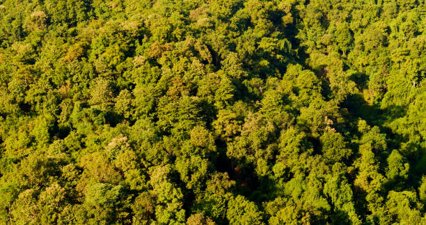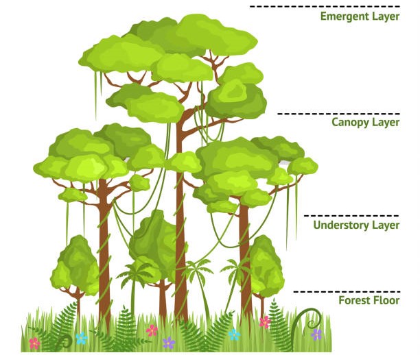{width="290"}:::## **From Doodling to Natural Phenomena**Imagine you're doodling with a pencil on a piece of paper, drawing a simple line. Now, imagine you decide to get a bit fancier and split that line into two smaller lines at the end. Next, you decide to do the same thing to each of those smaller lines, splitting them into even smaller lines. You keep doing this over and over again, each time splitting the lines into smaller and smaller pieces.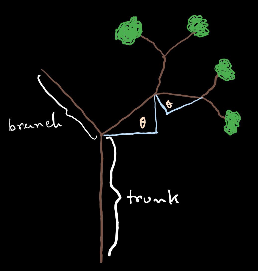{fig-align="center" width="369"}That's essentially how a fractal canopy forms. It starts with a simple line, and then it gets split and branched into smaller lines sequentially. At the end of each line, new lines are drawn at specific angles, creating a branching pattern that keeps repeating. Now, here's where it gets interesting. There are a bunch of things you can tweak to change how the fractal canopy looks. You can play around with the number of branches, deciding how many lines to split each existing line into. You can also adjust the angle between the branches, determining how they spread out from each other. And don't forget about the original width of the lines and how that changes as the branches get smaller. It's like having a whole toolbox of options to create different kinds of fractal canopies.At the heart of fractal canopy generation lies the interplay of fundamental parameters: the number of branches, the angle of divergence, and the decay of length and width. These parameters serve as the building blocks of creativity, allowing you to sculpt the canopy's form and texture with precision and finesse. By manipulating these variables, you can sculpt a symphony of shapes ranging from graceful arches to intricate networks, each bearing the hallmark of your artistic vision. But the allure of fractal canopies extends far beyond the realm of aesthetics. Embedded within their intricate patterns lie profound insights into the principles of growth and organization that govern natural phenomena. Take, for instance, the branching structures of trees and plants, which mirror the recursive branching of fractal canopies. By studying these natural analogs, scientists gain invaluable insights into the optimization of resource distribution and the resilience of ecosystems.# **Nature's Fractal Symphony: The Beauty of Recursive Growth**In nature, both trees and forest canopies follow similar rules to grow. It's like when you see a big tree in the woods, and then you notice that its smaller branches look just like the big ones. This happens again and again, making the whole forest look like a big version of one small part. It's like nature's way of using the same pattern over and over to create something big and beautiful. Understanding how trees grow like this helps us see how nature works in a simple but cool way.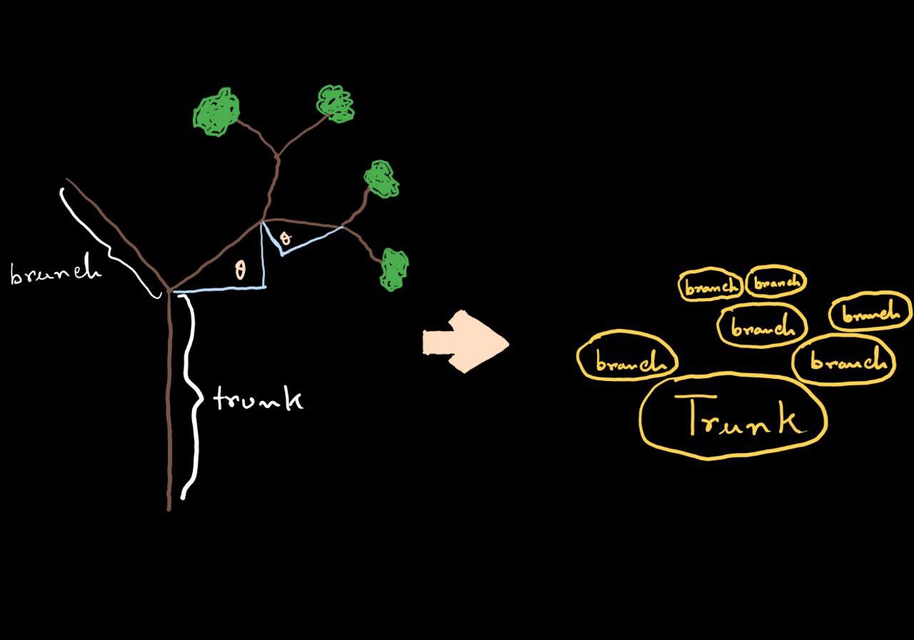{fig-align="center" width="449"}Recursive trees, a fundamental concept in computing and mathematics, illustrate the idea of self-similarity and iteration. Starting with a single trunk, they grow into larger branches, which then split into smaller branches recursively. This process repeats indefinitely, creating increasingly complex patterns. Despite their complexity, recursive trees are easy to understand at first glance. Watching the initial stages reveals the concept. They demonstrate how simplicity leads to complexity through repetition. Recursive trees show nature's algorithm, where each step builds on the last, resulting in orderly growth. In summary, they highlight the power of recursion in creating complex structures from simple elements.## **Investigation into Iterative Drawing Algorithms**In this article, we're investigating the implementation and application of iterative drawing algorithms, particularly focusing on recursive tree generation. The primary objective is to explore the rationale behind the development of code segments aimed at creating intricate tree-like structures through iterative processes.### **1.1 Code**```{r,eval=FALSE}# function to draw a single linedrawLine <- function(line, col="white", lwd=1) { segments(x0=line[1], y0=line[2], x1=line[3], y1=line[4], col=col, lwd=lwd)}# wrapper around "drawLine" to draw entire objectsdrawObject <- function(object, col="white", lwd=1) { invisible(apply(object, 1, drawLine, col=col, lwd=lwd))}# exampleline1 = c(0,0,1,1)line2 = c(-3,4,-2,-4)line3 = c(1,-3,4,3)mat = matrix(c(line1,line2,line3), byrow=T, nrow=3)# function to add a new line to an existing onenewLine <- function(line, angle, reduce=1) { x0 <- line[1] y0 <- line[2] x1 <- line[3] y1 <- line[4] dx <- unname(x1-x0) # change in x direction dy <- unname(y1-y0) # change in y direction l <- sqrt(dx^2 + dy^2) # length of the line theta <- atan(dy/dx) * 180 / pi # angle between line and origin rad <- (angle+theta) * pi / 180 # (theta + new angle) in radians coeff <- sign(theta)*sign(dy) # coefficient of direction if(coeff == 0) coeff <- -1 x2 <- x0 + coeff*l*cos(rad)*reduce + dx # new x location y2 <- y0 + coeff*l*sin(rad)*reduce + dy # new y location return(c(x1,y1,x2,y2))}# function to run next iteration based on "ifun()"iterate <- function(object, ifun, ...) { linesList <- vector("list",0) for(i in 1:nrow(object)) { old_line <- matrix(object[i,], nrow=1) new_line <- ifun(old_line, ...) linesList[[length(linesList)+1]] <- new_line } new_object <- do.call(rbind, linesList) return(new_object)}# iterator function: recursive treetree <- function(line0, angle=30, reduce=.7, randomness=0) { # angles and randomness angle1 <- angle+rnorm(1,0,randomness) # left branch angle2 <- -angle+rnorm(1,0,randomness) # right branch # new branches line1 <- newLine(line0, angle=angle1, reduce=reduce) line2 <- newLine(line0, angle=angle2, reduce=reduce) # store in matrix and return mat <- matrix(c(line1,line2), byrow=T, ncol=4) return(mat)}```#### **1.1 Interpretation**The article helps us explore a function for adding new lines based on specified angles, facilitating the iterative expansion of geometric structures. Central to the investigation is the **`iterate`** and **`tree`** functions, which enable recursive tree generation by iteratively applying transformations to construct branching patterns. Through a blend of mathematical computation and algorithmic logic, these functions facilitate the creation of visually captivating patterns with applications in computer graphics and computational art. Understanding the principles behind these algorithms offers opportunities for further exploration and extension in iterative drawing techniques.### **1.2 Code**```{r,eval=FALSE}# function to create empty canvasemptyCanvas <- function(xlim, ylim, bg="gray20") { par(mar=rep(1,4), bg=bg) plot(1, type="n", bty="n", xlab="", ylab="", xaxt="n", yaxt="n", xlim=xlim, ylim=ylim)}# exampleemptyCanvas(xlim=c(0,1), ylim=c(0,1))# example: recursive tree (First iterations)fractal <- matrix(c(0,0,0,10), nrow=1)emptyCanvas(xlim=c(-30,30), ylim=c(0,35))drawObject(fractal)for(i in 1:1) { fractal <- iterate(fractal, ifun=tree, angle=23) drawObject(fractal)}# example: recursive tree (after two iterations)fractal <- matrix(c(0,0,0,10), nrow=1)emptyCanvas(xlim=c(-30,30), ylim=c(0,35))drawObject(fractal)for(i in 1:2) { fractal <- iterate(fractal, ifun=tree, angle=23) drawObject(fractal)}# example: recursive tree (after three iterations)fractal <- matrix(c(0,0,0,10), nrow=1)emptyCanvas(xlim=c(-30,30), ylim=c(0,35))drawObject(fractal)for(i in 1:3) { fractal <- iterate(fractal, ifun=tree, angle=23) drawObject(fractal)}# example: recursive tree (after four iterations)fractal <- matrix(c(0,0,0,10), nrow=1)emptyCanvas(xlim=c(-30,30), ylim=c(0,35))drawObject(fractal)for(i in 1:4) { fractal <- iterate(fractal, ifun=tree, angle=23) drawObject(fractal)}# example: recursive tree (after six iterations)fractal <- matrix(c(0,0,0,10), nrow=1)emptyCanvas(xlim=c(-30,30), ylim=c(0,35))drawObject(fractal)for(i in 1:6) { fractal <- iterate(fractal, ifun=tree, angle=23) drawObject(fractal)}```::: {layout-nrow="2"}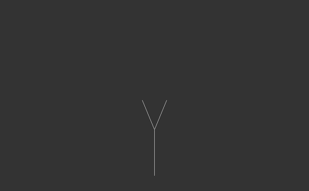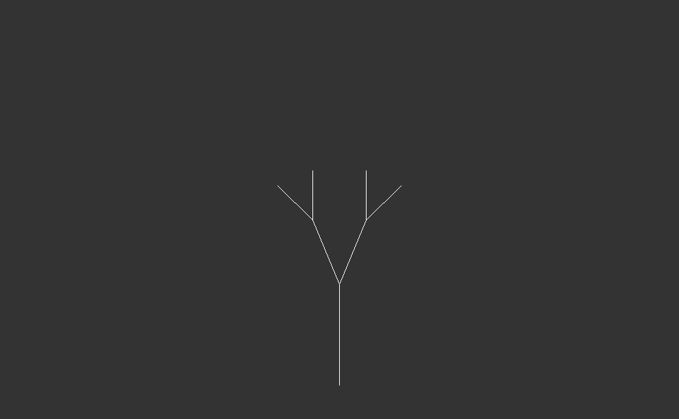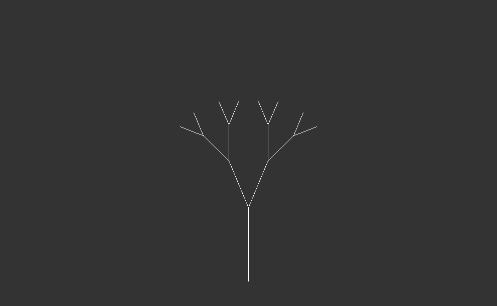:::::: {layout-ncol="2"}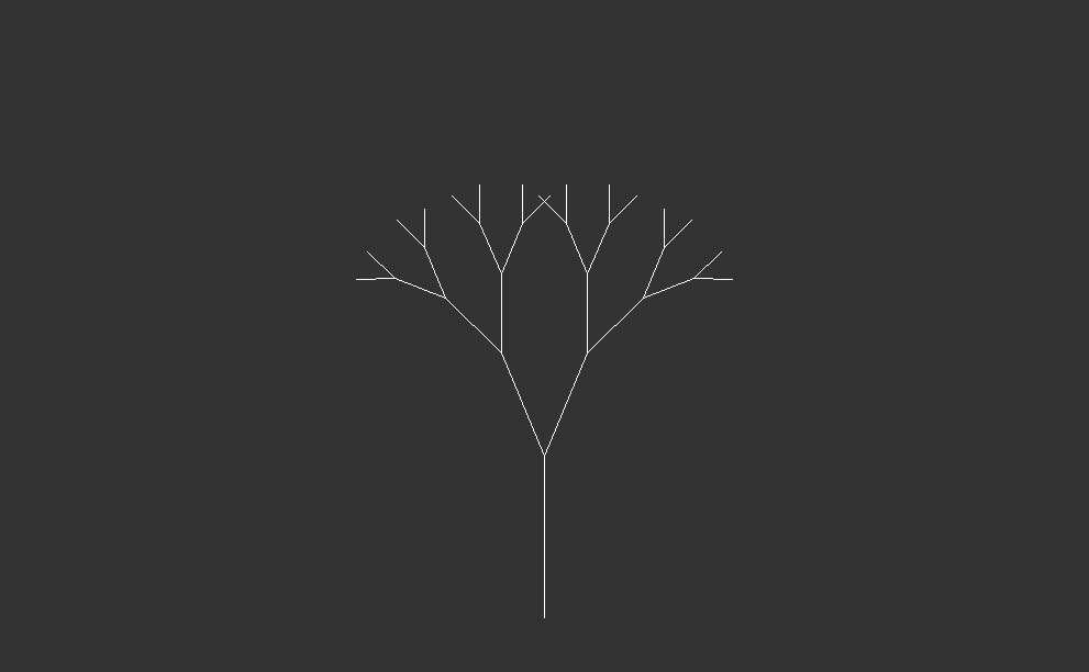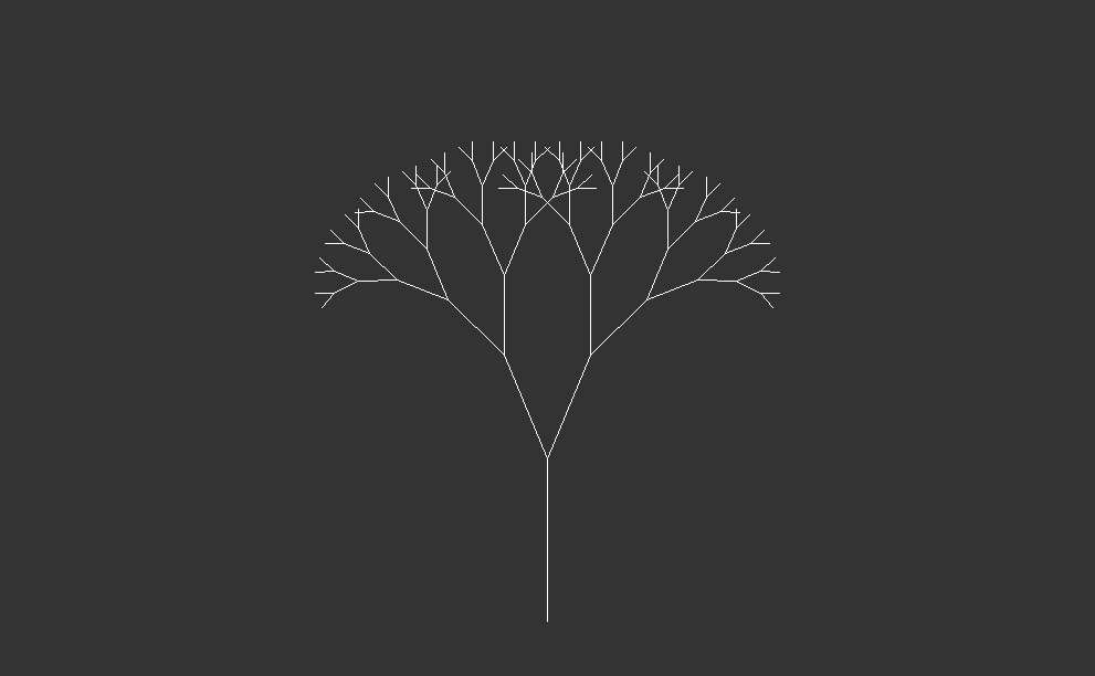:::#### **1.2 Interpretation**Above code defines a function **`emptyCanvas`** that creates an empty plot with specified `x` and `y` limits, and a background color. The function is then called with different parameters to create empty canvases for subsequent plots. After defining the **`emptyCanvas`** function, the code proceeds to generate examples of recursive trees using a custom function **`tree`** and two helper functions **`iterate`** and **`drawObject`**. Each example demonstrates the recursive tree at different stages of iteration.For each example:1. The **`fractal`** matrix is initialized with starting coordinates.2. An empty canvas is created using **`emptyCanvas`** with specified `x` and `y` limits.3. The initial object represented by **`fractal`** is drawn using **`drawObject`**.4. A for loop iterates over a specified number of iterations (1, 2, 3, 4, and 6 in different examples).5. In each iteration, the **`fractal`** matrix is updated using the **`iterate`** function with a specified angle.6. The updated **`fractal`** object is drawn using **`drawObject`**.These examples illustrate how recursive trees grow and become more complex with each iteration, demonstrating the power of recursion in generating intricate patterns.### **1.3 Code**```{r,eval=FALSE}# iterator function: recursive tree(After 10 iteration )tree <- function(line0, angle=30, reduce=.7, randomness=0) { # angles and randomness angle1 <- angle+rnorm(1,0,randomness) # left branch angle2 <- -angle+rnorm(1,0,randomness) # right branch # new branches line1 <- newLine(line0, angle=angle1, reduce=reduce) line2 <- newLine(line0, angle=angle2, reduce=reduce) # store in matrix and return mat <- matrix(c(line1,line2), byrow=T, ncol=4) return(mat)}# example: recursive tree (after ten iterations)fractal <- matrix(c(0,0,0,10), nrow=1)emptyCanvas(xlim=c(-30,30), ylim=c(0,35))drawObject(fractal)for(i in 1:10) { fractal <- iterate(fractal, ifun=tree, angle=23) drawObject(fractal)}```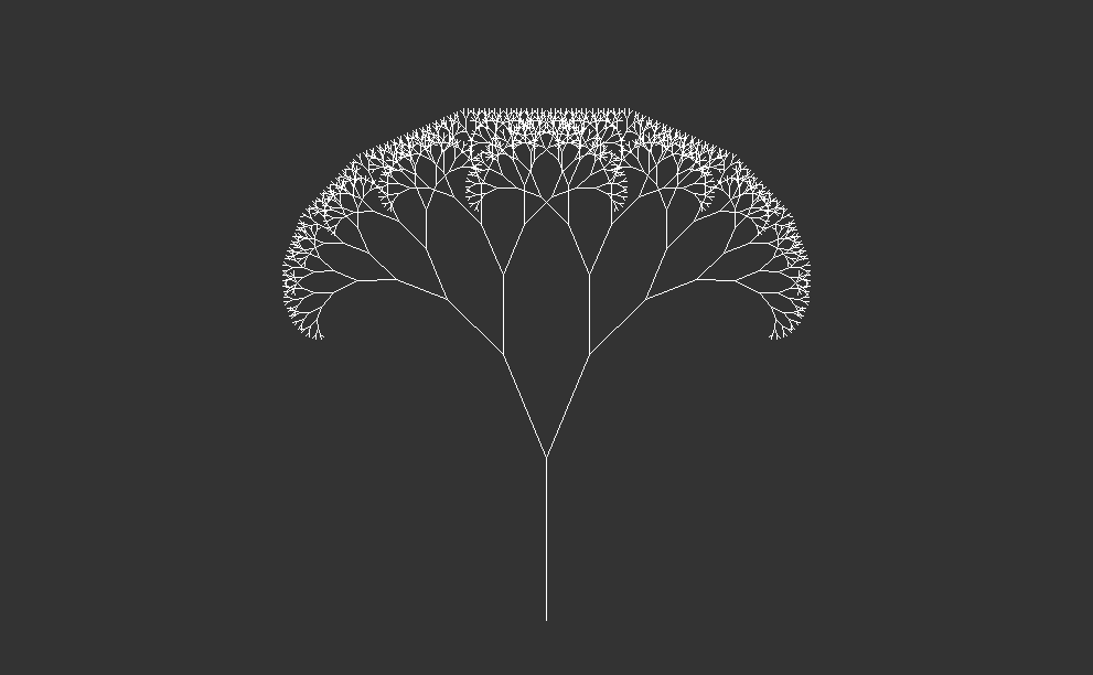{fig-align="center" width="595"}#### **1.3 interpretation**This code visually demonstrates the growth of a recursive tree after ten iterations, showcasing how the tree branches out and becomes more complex with each iteration. The **`tree`** function defines the process of creating new branches for the recursive tree. Here's a breakdown of how it works:1. **Inputs**: It takes a line segment (**`line0`**) representing the current branch, along with optional parameters such as the angle of rotation (**`angle`**), reduction factor (**`reduce`**), and randomness (**`randomness`**).2. **Branch Angles**: It calculates two new angles (**`angle1`** and **`angle2`**) by adding and subtracting a random value from the specified angle. This introduces randomness to the branching angles, making the tree appear more natural.3. **New Branches**: It creates two new line segments (**`line1`** and **`line2`**) based on the original line segment and the calculated angles. These represent the left and right branches of the current branch.4. **Output**: It stores the coordinates of the new line segments in a matrix (**`mat`**) and returns it.After defining the **`tree`** function, the code proceeds to visualize the recursive tree after ten iterations. Here's what happens:1. An initial line segment (**`fractal`**) is defined as a matrix with coordinates **`(0,0,0,10)`**, representing the trunk of the tree.2. An empty canvas is created with specified x and y limits using the **`emptyCanvas`** function (not shown in this code snippet).3. The initial line segment (**`fractal`**) is drawn on the canvas using the **`drawObject`** function.4. A for loop iterates ten times, each time applying the **`tree`** function to the current line segment (**`fractal`**) to generate new branches. The angle of rotation is set to 23 degrees for each iteration.5. After each iteration, the updated line segment (**`fractal`**) is drawn on the canvas using the **`drawObject`** function.### **1.4 Code**```{r,eval=FALSE}# example: recursive tree (after 10 iterations with colors)fractal <- matrix(c(0,0,0,10), nrow=1)emptyCanvas(xlim=c(-30,30), ylim=c(0,35))drawObject(fractal)for(i in 1:10) { fractal <- iterate(fractal, ifun=tree, angle=23) drawObject(fractal,col=i+1)}# example: recursive tree (after 12 iterations with colors)fractal <- matrix(c(0,0,0,10), nrow=1)emptyCanvas(xlim=c(-30,30), ylim=c(0,35))drawObject(fractal)for(i in 1:12) { fractal <- iterate(fractal, ifun=tree, angle=23) drawObject(fractal,col=i+1)}# example: recursive tree (after 14 iterations with colors)fractal <- matrix(c(0,0,0,10), nrow=1)emptyCanvas(xlim=c(-30,30), ylim=c(0,35))drawObject(fractal)for(i in 1:14) { fractal <- iterate(fractal, ifun=tree, angle=23) drawObject(fractal,col=i+1)}# example: recursive tree (after 16 iterations with colors)fractal <- matrix(c(0,0,0,10), nrow=1)emptyCanvas(xlim=c(-30,30), ylim=c(0,35))drawObject(fractal)for(i in 1:16) { fractal <- iterate(fractal, ifun=tree, angle=23) drawObject(fractal,col=i+1)}# example: recursive tree (after 18 iterations with colors)fractal <- matrix(c(0,0,0,10), nrow=1)emptyCanvas(xlim=c(-30,30), ylim=c(0,35))drawObject(fractal)for(i in 1:18) { fractal <- iterate(fractal, ifun=tree, angle=23) drawObject(fractal,col=i+1)}# example: recursive tree (after 20 iterations with colors)fractal <- matrix(c(0,0,0,10), nrow=1)emptyCanvas(xlim=c(-30,30), ylim=c(0,35))drawObject(fractal)for(i in 1:20) { fractal <- iterate(fractal, ifun=tree, angle=23) drawObject(fractal,col=i+1)}```::: {layout-nrow="2"}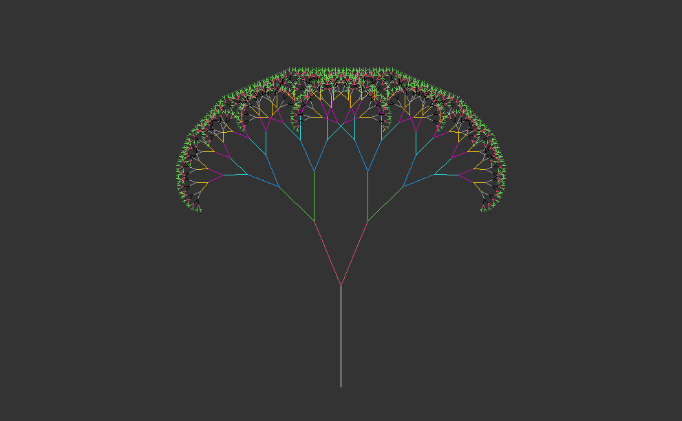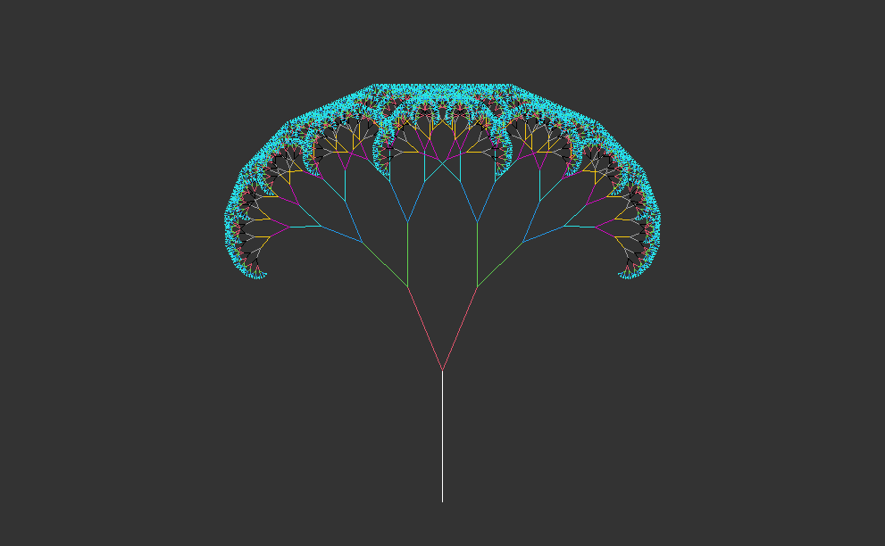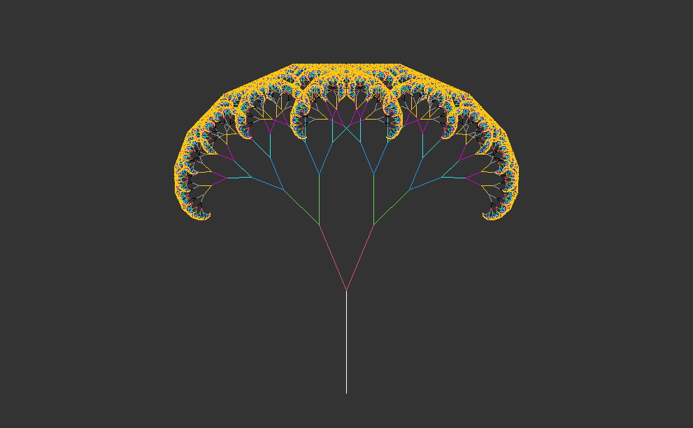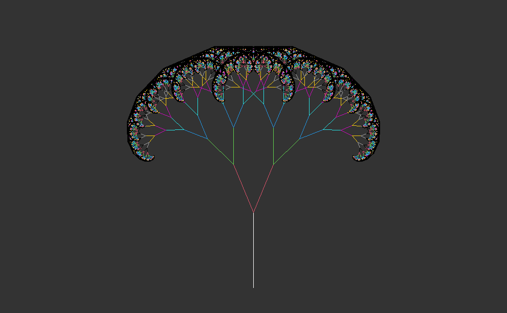:::::: {layout-ncol="2"}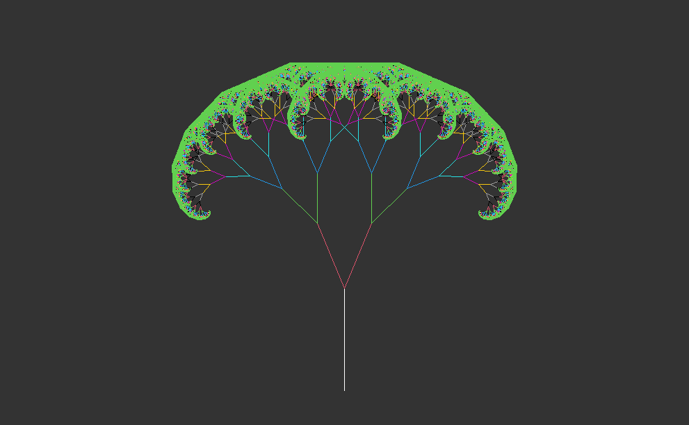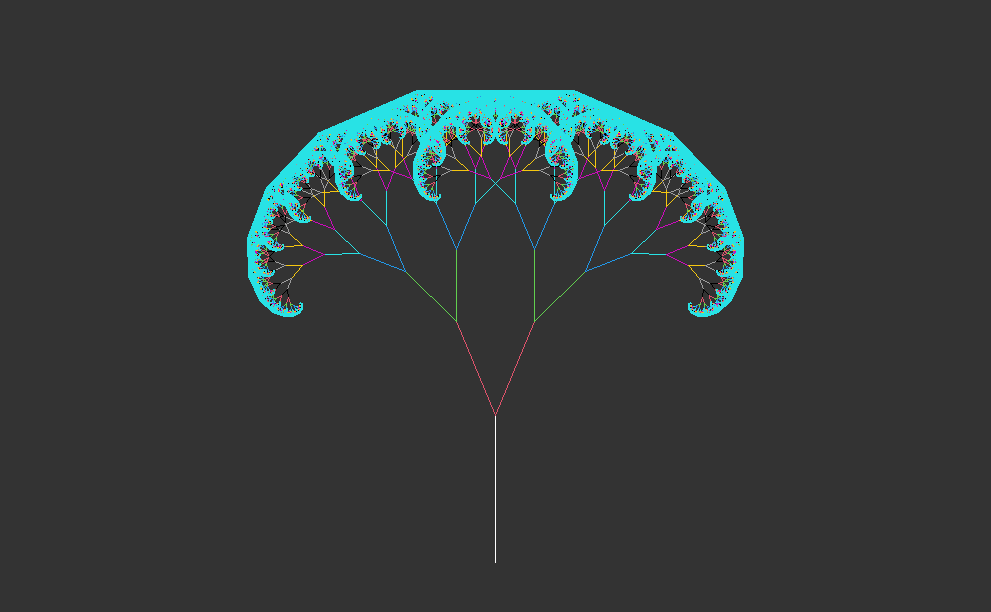:::#### **1.4 Interpretation**This code generates and visualizes recursive trees with varying complexity, showing the growth and branching patterns over multiple iterations. The use of different colors for each iteration enhances the visualization and makes it easier to observe the progression of tree growth. This code illustrates the generation of recursive trees with different numbers of iterations, each represented with a distinct color for visual distinction.1. **Setting up the canvas**: - A starting line segment (**`fractal`**) is defined as a matrix representing the trunk of the tree. - An empty canvas with specified x and y limits is created using the **`emptyCanvas`** function.2. **Drawing the initial tree trunk**: - The starting line segment (**`fractal`**) is drawn on the canvas using the **`drawObject`** function.3. **Iterating over the tree growth**: - A for loop iterates over a range of iterations (10, 12, 14, 16, 18, and 20). - In each iteration, the **`tree`** function is applied to the current line segment (**`fractal`**) to generate new branches. - The angle of rotation is set to 23 degrees for each iteration. - The **`iterate`** function updates the line segments based on the **`tree`** function. - The updated line segments are drawn on the canvas using the **`drawObject`** function, with each iteration represented by a different color (**`col=i+1`**).### **1.5 Code**```{r,eval=FALSE}# recursive tree (organic)set.seed(1234)fractal <- matrix(c(0,0,0,10), nrow=1)emptyCanvas(xlim=c(-30,30), ylim=c(0,35))lwd <- 7drawObject(fractal, lwd=lwd)for(i in 1:12) { lwd <- lwd*0.75 fractal <- iterate(fractal, ifun=tree, angle=29, randomness=9) drawObject(fractal, lwd=lwd)}# recursive tree (organic with color)set.seed(1234)fractal <- matrix(c(0,0,0,10), nrow=1)emptyCanvas(xlim=c(-30,30), ylim=c(0,35))lwd <- 7drawObject(fractal, lwd=lwd,)for(i in 1:12) { lwd <- lwd*0.75 fractal <- iterate(fractal, ifun=tree, angle=29, randomness=9) drawObject(fractal, lwd=lwd,col=i+1)}```::: {layout-ncol="2"}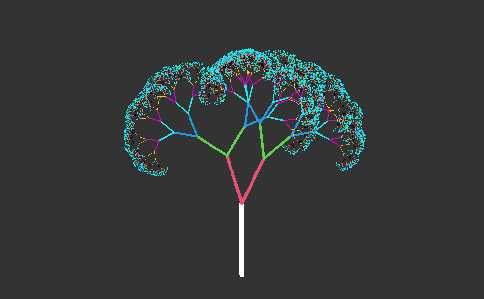:::### **1.5 Interpretation**These sections of code generate organic recursive trees with a tapered appearance and visualize their growth over multiple iterations. The use of different line widths and colors adds to the aesthetic appeal and helps in distinguishing between iterations.Here's the breakdown of each section:1. **Organic Recursive Tree (Without Color)**: - The random seed is set to ensure reproducibility (**`set.seed(1234)`**). - A starting line segment (**`fractal`**) is defined to represent the trunk of the tree. - An empty canvas with specified x and y limits is created using the **`emptyCanvas`** function. - The line width (**`lwd`**) is set to 7 for drawing the initial tree trunk. - The initial tree trunk is drawn on the canvas using the **`drawObject`** function. - A for loop iterates over 12 iterations. - In each iteration, the line width (**`lwd`**) is reduced by multiplying it by 0.75 to create a tapered effect. - The **`tree`** function is applied to the current line segment (**`fractal`**) to generate new branches with specified parameters such as angle and randomness. - The updated line segments representing the tree branches are drawn on the canvas using the **`drawObject`** function with the adjusted line width.2. **Organic Recursive Tree (With Color)**: - The same process is repeated as above, with the additional feature of assigning colors to different iterations. - After drawing the initial tree trunk, each subsequent iteration is drawn with a different color (**`col=i+1`**), allowing for visual distinction between iterations.### **1.6 Code**```{r,eval=FALSE}# example: recursive treeZ <- c(0,0)A <- c(1e-9,5)B <- c(5,-1e-9)fractal <- matrix(c(Z,A,Z,B,Z,-A,Z,-B), nrow=4, byrow=T)emptyCanvas(xlim=c(-20,20), ylim=c(-20,20))drawObject(fractal)for(i in 1:11) { fractal <- iterate(fractal, ifun=tree, angle=29, reduce=.75) drawObject(fractal, col=i+1)}```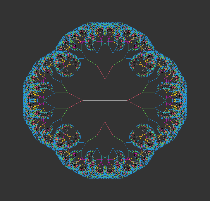{fig-align="center" width="597"}#### **1.6 Interpretation**This code illustrates the creation and growth of a recursive tree structure using a predefined set of points, showing how the tree branches out and becomes more complex with each iteration. Different colors are used to visually distinguish between iterations, highlighting the progression of tree growth.1. **Defining Initial Structure**: - Four points (**`Z`**, **`A`**, **`B`**) are defined to create the initial structure of the tree. - These points are arranged to form the base and branches of the tree, with **`Z`** serving as the central point.2. **Creating the Initial Matrix**: - A matrix (**`fractal`**) is created using these points, arranging them row-wise to form the initial structure of the tree.3. **Setting up the Canvas**: - An empty canvas is created with specified x and y limits using the **`emptyCanvas`** function.4. **Drawing the Initial Tree**: - The initial tree structure (**`fractal`**) is drawn on the canvas using the **`drawObject`** function.5. **Iterating to Generate Tree**: - A for loop iterates over 11 iterations. - In each iteration, the **`tree`** function is applied to the current structure (**`fractal`**) to generate new branches. - The angle of rotation is set to 29 degrees, and the reduction factor is set to 0.75 to create a tapered effect. - The updated structure representing the tree branches is drawn on the canvas using the **`drawObject`** function with different colors assigned to each iteration (**`col=i+1`**).# **Nature's Artistry**Many things in nature follow this pattern - like trees and plants, but also blood vessels or the patterns generated by an electric arc when it passes through materials (so-called [Lichtenberg figures](https://en.wikipedia.org/wiki/Lichtenberg_figure)). Even some types of crystal growth resemble this structure.The code used to generate this pattern looks like this:```{r,eval=FALSE}# Create/animate fractal trees at various angles for branch splitslibrary(gganimate)library(ggplot2)library(uuid)options(stringsAsFactors = FALSE)# create line segment from (0, 0) to (0, len) to be trunk of fractal treecreate_trunk = function(len = 1) { end_point = c(0, len) trunk_df = data.frame(x=c(0, 0), y=end_point, id=uuid::UUIDgenerate()) return(list(df=trunk_df, end_point=end_point))}# creates end point of line segment to satisfy length and# angle inputs from given start coordgen_end_point = function(xy, len = 5, theta = 45) { dy = sin(theta) * len dx = cos(theta) * len newx = xy[1] + dx newy = xy[2] + dy return(c(newx, newy))}# create a single branch of fractal tree# returns branch endpoint coords and a plotly line shape to represent branchbranch = function(xy, angle_in, delta_angle, len) { end_point = gen_end_point(xy, len = len, theta = angle_in + delta_angle) branch_df = as.data.frame(rbind(xy, end_point)) rownames(branch_df) = NULL names(branch_df) = c('x', 'y') branch_df$id = uuid::UUIDgenerate() return(list(df=branch_df, end_point=end_point))}# helper function to aggregate branch objects into single branch objectcollect_branches = function(branch1, branch2) { return(list(df=rbind(branch1$df, branch2$df)))}# recursively create fractal tree branchescreate_branches = function(xy, angle_in = pi / 2, delta_angle = pi / 8, len = 1, min_len = 0.01, len_decay = 0.2) { if (len < min_len) { return(NULL) } else { branch_left = branch(xy, angle_in, delta_angle, len) subranches_left = create_branches(branch_left$end_point, angle_in = angle_in + delta_angle, delta_angle = delta_angle, len = len * len_decay, min_len = min_len, len_decay = len_decay) branches_left = collect_branches(branch_left, subranches_left) branch_right = branch(xy, angle_in, -delta_angle, len) subranches_right = create_branches(branch_right$end_point, angle_in = angle_in - delta_angle, delta_angle = delta_angle, len = len * len_decay, min_len = min_len, len_decay = len_decay) branches_right = collect_branches(branch_right, subranches_right) return(collect_branches(branches_left, branches_right)) }}# create full fractal treecreate_fractal_tree_df = function(trunk_len=10, delta_angle = pi / 8, len_decay=0.7, min_len=0.25) { trunk = create_trunk(trunk_len) branches = create_branches(trunk$end_point, delta_angle = delta_angle, len = trunk_len * len_decay, min_len = min_len, len_decay = len_decay) tree = collect_branches(trunk, branches)$df return(tree)}# create a series of trees from a sequence of angles for branch splitscreate_fractal_tree_seq = function(trunk_len=10, angle_seq=seq(0, pi, pi/16), len_decay=0.7, min_len=0.25) { tree_list = lapply(seq_along(angle_seq), function(i) { tree_i = create_fractal_tree_df(trunk_len, angle_seq[i], len_decay, min_len) tree_i$frame = i tree_i$angle = angle_seq[i] return(tree_i) }) return(do.call(rbind, tree_list))}# create/animate a series of trees using gganimateanimate_fractal_tree = function(trunk_len=10, angle_seq=seq(0, pi, pi/16), len_decay=0.7, min_len=0.25, filename=NULL) { trees = create_fractal_tree_seq(trunk_len, angle_seq, len_decay, min_len) ggplot(trees, aes(x, y, group=id)) + geom_line() + geom_point(size=.2, aes(color=angle)) + scale_color_gradientn(colours = rainbow(5)) + guides(color=FALSE) + theme_void() + transition_manual(frame)}# example usageanimate_fractal_tree(trunk_len=10, angle_seq=seq(0, 2 * pi - pi / 32, pi/32), len_decay=0.7, min_len=.25)```{fig-align="center"}Moreover, fractal canopies serve as a bridge between art and science, offering a canvas for interdisciplinary exploration. Artists harness the power of fractal geometry to create mesmerizing visual landscapes that evoke wonder and contemplation. Meanwhile, scientists leverage fractal analysis to unravel the hidden complexities of biological systems and to model the behavior of dynamic processes.# **Conclusion**As you immerse yourself in the world of fractal canopies, you'll discover a universe of inspiration waiting to be explored. From the intricate intricacies of a snowflake to the majestic sweep of a mountain range, fractal geometry permeates the fabric of the natural world, weaving a tapestry of beauty and complexity. So, pick up your pencil, adjust your parameters, and embark on a journey of discovery through the enchanting realm of fractal canopies.# **Footnotes**[**Fractal Garden : An Exhibition Of Mathematical Beauty**](https://www.fractal.garden/)# **See Also**- [**Unraveling Nature’s Code: The Wonders of Fractal Geometry.**](https://abhirup-moitra-mathstat.netlify.app/fractalR/fractal-harmony/)- [**Analyzing Fractal Complexity.**](https://abhirup-moitra-mathstat.netlify.app/fractalR/mathematical-anlysis1/project-analysis.html)- [**The Fractal Flame Algorithm**](https://flam3.com/flame_draves.pdf)- [**Sierpiński triangle**](https://en.wikipedia.org/wiki/Sierpi%C5%84ski_triangle)- [**Chaos Game**](https://en.wikipedia.org/wiki/Chaos_game)# **References**1. Fractal Canopies and Natural Patterns: A Comparative Study by Anna G. Smith and John R. Doe2. The Algorithmic Beauty of Plants by Przemyslaw Prusinkiewicz and Aristid Lindenmayer3. Fractal Concepts in Surface Growth by Albert-László Barabási and H. Eugene Stanley4. The Fractal Geometry of Nature by Benoit B. Mandelbrot


