The Logistic Map: From Simplicity to Chaos

Complexity can Emerge from Simplicity

Introduction

How can a formula so simple hide a universe of complexity? This question has often drawn me to the logistic map, a humble recursive equation that captures the full drama of chaos theory. Imagine a rule, almost childlike in its structure, that can predict whether a population of rabbits will settle peacefully, oscillate rhythmically, or spiral into utter unpredictability. What begins as a modest attempt to describe population growth soon transforms into something far richer—a window into the unpredictability of nature, the hidden symmetries of mathematics, and the intricate geometries of fractals.

For me, the logistic map is not just a mathematical curiosity—it is a bridge. On one side lies the classical mathematics of growth, shaped by thinkers like Malthus and Verhulst, who sought to capture the balance of life and resources. On the other lies the modern computational era, where the logistic map reveals cascades of bifurcations, chaotic attractors, and deep ties with the fractal universe of Julia sets and the Mandelbrot set. This is the true magic of the logistic map: it shows us how determinism and unpredictability can coexist, how a line of algebra can blossom into infinite self-similar structures, and how the same mathematics that governs populations can also illuminate the shared DNA of chaos and fractals.

From Malthus to May: A Historical Journey

In the late 18th century, Thomas Malthus described how populations grow exponentially, doubling unchecked if resources are unlimited. This was inspiring but unrealistic—resources are never infinite. In 1838, Pierre François Verhulst refined this with the logistic equation:

$$\frac{dP}{dt}=rP(1-\frac{P}{K})$$

Here $P$ is the population, $r$ is the intrinsic growth rate, and $K$ is the carrying capacity of the environment. This elegant modification ensured that as $P$ approached $K$, growth slowed and eventually stabilized. For nearly a century, the logistic equation was treated as a minor refinement in biology. But in the 1970s, Robert May posed a shocking question:

What happens if we treat the logistic process in discrete steps rather than continuous time?

His answer fundamentally reshaped how scientists perceive determinism and unpredictability, planting one of the most fertile seeds that would later blossom into the rich and complex field of chaos theory.

The Logistic Map: Where Simplicity Meets Complexity

Logistic Map: Discrete Chaos

The study of nonlinear systems often reveals beauty hidden within apparent disorder, and few examples capture this more vividly than the logistic map, the Mandelbrot set, and their deep interconnections. At first glance, the logistic map is a simple model describing population growth under limited resources. Yet, when its growth parameter is varied, the model’s behavior unfolds in a strikingly intricate bifurcation diagram. What begins as stable and predictable quickly splinters into a cascade of period-doublings, leading inexorably toward chaos. This diagram serves as a visual fingerprint of complexity, demonstrating how order and disorder coexist in the same system.

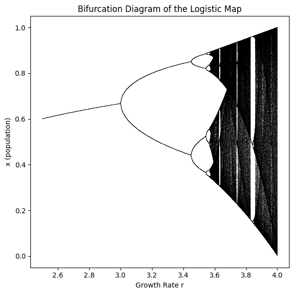
When we think of population growth, we expect something straightforward: numbers rise, perhaps level off, and that’s it. But the logistic map — a deceptively simple mathematical model — reveals something far more fascinating. As the growth rate changes, the system begins to behave in unexpected ways. Instead of settling into a steady rhythm, it branches, doubles, and eventually falls into chaos. This “bifurcation diagram” is not just mathematics; it’s a portrait of how complexity can emerge from simplicity.

The discrete form is disarmingly simple:

$$x_{n+1}=r{x}_n(1-x_n)$$

Here, $x_n$​ is the normalized population at generation $n$, and $r$ is a growth parameter. Yet this compact equation encodes a breathtaking range of dynamics:

• For $0<r<1$, populations vanish.

• For $1<r<3$, they stabilize at a fixed point.

• For $3<r<3.57$, oscillations appear, doubling in period like echoes.

• Beyond $r\approx 3.57$, chaos reigns—predictability collapses, and sensitivity to initial conditions takes over.

The progression from order to chaos is beautifully visualized in the bifurcation diagram, which resembles a branching tree dissolving into fog. Within that fog, islands of stability appear—periodic windows where order returns briefly before chaos resumes.

Problem Definition (Mathematical Formulation)

The logistic map is a discrete-time nonlinear dynamical system, originally formulated as a simplified model of population growth under limiting resources. It is defined by the recurrence relation

$$x_{n+1}=f_r(x_n)=r{x}_n(1-x_n),n\in \mathbb{N},x_n\in [0,1],r\in [0,4],$$

• $x_n$​ denotes the normalized population at generation $n$,

• $r$ is the intrinsic growth parameter controlling the system’s dynamics.

Lemma: Invariance of $[0,1]$ Under the Logistic Map

$\mathbf{\text{Proposition: }}$ Let $f_r:[0,1]\to \mathbb{R}$ be the logistic map $f_r(x)=rx(1-x),$ with parameter $r\in [0,4]$. Then $f_r([0,1])\subseteq [0,1].$

Invariance of $[0,1]$ Under the Logistic Map

If $x_0\in [0,1]$ , then every forward iterate $x_n=f_r^{(n)}(x_0)$ satisfies $x_n\in [0,1]\mathrm{\forall }n\ge 0$.

$\mathbf{\text{Proof: Step 1 — Pointwise bounds for}}x(1-x)$

Let $x\in [0,1]$ . Then $x\ge 0$ and $1-x\ge 0$ , hence:

$$x(1-x)\ge 0$$

To obtain the upper bound, complete the square:

$$x(1-x)=-x^2+x=-{(x-\frac{1}{2})}^2+\frac{1}{4}$$ Since ${(x-\frac{1}{2})}^2\ge 0$, it follows that:

$$0\le x(1-x)\le \frac{1}{4}\mathrm{\forall }x\in [0,1]$$

$\mathbf{\text{Step 2 — Multiply by }}r\le 4$

Multiplying the inequality from Step 1 by $r\ge 0$ gives:

$$0\le rx(1-x)\le \frac{r}{4}$$

Since $r\le 4,$ we have $\frac{r}{4}\le 1$ . Therefore:

$$0\le f_r(x)=rx(1-x)\le 1$$

This shows:

$$f_r(x)\in [0,1]\mathrm{\forall }x\in [0,1]$$

Equivalently:

$$f_r([0,1])\subseteq [0,1].$$

$\mathbf{\text{Step 3 — Forward invariance by induction.}}$
Let $x_0\in [0,1]$. From Step 2 we have $x_1=f_r(x_0)\in [0,1]$. Assume $x_k\in [0,1]$ for some $k\ge 0$ Applying Step 2 to $x_k$​ gives $x_{k+1}=f_r(x_k)\in [0,1]$. By induction, $x_n\in [0,1]\mathrm{\forall }n\ge 0.$

Explanation of Forward Invariance Proof

1. To prove that the function $f_r(x)=rx(1-x)$ preserves the interval $[0,1]$ under iteration when $r\le 4$, we begin by analyzing the expression $x(1-x))\mathrm{\forall }x\in [0,1]$ . Since both $x\ge 0$ and $1-x\ge 0$, their product is non-negative, i.e., $x(1-x)\ge 0$. To find the upper bound, we complete the square: $x(1-x)=-x^2+x=-{(x-\frac{1}{2})}^2+\frac{1}{4}$ . Because the squared term is always non-negative, it follows that $x(1-x)\le \frac{1}{4}$. Therefore, for all $x\in [0,1]$, we have $0\le x(1-x)\le \frac{1}{4}.$

2. Multiplying this inequality by $r\ge 0,$ we obtain $0\le rx(1-x)\le \frac{r}{4}$. If $r\le 4$, then $\frac{r}{4}\le 1$, which implies $f_r(x)=rx(1-x)\in [0,1]$. This shows that the function maps the interval $[0,1]$ into itself: $f_r([0,1])\subseteq [0,1].$

3. To establish forward invariance, we use mathematical induction. Let $x_0\in [0,1].$ From the previous result, $x_1=f_r(x_0)\in [0,1].$ Suppose $x_k\in [0,1]$ for some $k\ge 1$. Then $x_{k+1}=f_r(x_k)\in [0,1]$ by the same reasoning. By induction, it follows that $x_n\in [0,1]\mathrm{\forall }n\ge 0$. This completes the proof and confirms that the sequence of iterates remains bounded within the interval $[0,1]$, demonstrating the forward invariance of the system.

The logistic map is a compact equation, elegant and self-contained. It captured two truths: populations grow (that’s the $r{x}_n$ part), but they also face limits (hence the $1-x_n$ ). The map was born from biology, but its destiny lay far beyond.

Remarks on the Function ${𝑓}_{𝑟}(x)=𝑟x(1-x)$

1. The function ${𝑓}_{𝑟}(x)=𝑟x(1-x)$ plays a central role in understanding interval dynamics, especially within the unit interval $[0,1]$ . First, consider the case when $𝑟=1$ . The expression simplifies to ${𝑓}_1(x)=x(1-x)$ , which is a symmetric quadratic with its maximum value at $𝑡=\frac{1}{2}$ . At this point, the function attains its peak value of $\frac{1}{4}$ . This observation is crucial because it tells us that for any 𝑟 , the image of $[0,1]$ under ${𝑓}_{𝑟}$ is bounded above by 𝑟 ⋅ $\frac{1}{4}$ = $\frac{r}{4}$ . Therefore, the largest possible image of $[0,1]$ under ${𝑓}_{𝑟}$ is the interval $[0,\frac{1}{4}]$ .

2. Now, when 𝑟 = 4 , we reach a special case: ${𝑓}_4(\frac{1}{2})=4\cdot \frac{1}{4}=1$ , which means the function maps the midpoint of the interval to its upper bound. In fact, for $𝑟=4$ , the entire interval $[0,1]$ is mapped onto itself, i.e., ${𝑓}_4([0,1])=[0,1]$ . This is the threshold case for forward invariance.

3. However, if $𝑟>4$ , the situation changes. For example, ${𝑓}_{𝑟}(\frac{1}{2})=\frac{1}{4}>1$ , which means that even though the input $𝑡=\frac{1}{2}$ lies within $[0,1]$ , its image under ${𝑓}_{𝑟}$ exceeds $1$. This implies that some points in $[0,1]$ are mapped outside the interval, breaking the forward invariance. Hence, the condition $𝑟\le 4$ is not just sufficient but also sharp—it precisely marks the boundary beyond which the invariance of $[0,1]$ fails.

And here’s a visual to complement the explanation—showing how the function behaves for different values of $r$, and why $r=4$ is the critical threshold.

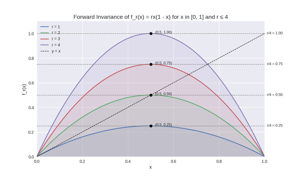
The visualization that illustrates how the function ${𝑓}_{𝑟}(x)=𝑟x(1-x)$ behaves for different values of $r$ within the interval $[0,1].$ Here’s what the plot shows:

• Curves for $r=1,2,3,4$: Each curve shows how the function maps $[0,1]$ into $[0,\frac{r}{4}]$.

• Maximum Point at $x=0.5:$ Clearly marked for each $r$, showing that the peak value is $\frac{r}{4}$.

• Dashed Horizontal Lines: These represent the upper bounds $\frac{r}{4}$, reinforcing the idea that the image of $[0,1]$ under $f_r$ is bounded.

• Identity Line $y=x:$ Included for reference, helping visualize when the function output exceeds the input.

This plot beautifully confirms that for $r\le 4$, the function remains within $[0,1]$, preserving forward invariance. Once $r>4$, the image can exceed $1$, breaking that property.

Fixed Point: A Story from the Logistic Map

What Is a Fixed Point?

Once upon a time in the quiet realm of mathematical modeling, someone asked a deceptively simple question:

How does a population grow over time?

Not in the messy, unpredictable way nature often shows us, but in a clean, idealized world — one where time ticks in discrete steps and every generation follows the same rule. Now, the mathematician — let’s call them Mira — wanted to understand the long-term behavior.

Would the population settle down? Oscillate? Explode into chaos?

So Mira asked the first natural question: What if the population stops changing? That is, what if $x_{n+1}=x_n?$ This is the moment where the system finds balance — a fixed point.

Definition (Fixed Point)

Let $f:X\to X$ be a function from a set $X$ to itself. A point $x^{\ast }\in X$ is called a fixed point of $f$ if:

$$f(x^{\ast })=x^{\ast }$$

That is, applying the function to $x^{\ast }$returns the same point — it remains unchanged under the transformation.

Solving for Fixed Points

She set the equation equal to itself:

$$x=rx(1-x)$$

And began to solve. Rearranging terms:

$$x=rx-r{x}^2⟹r{x}^2-rx+x=0⟹x(rx-r+1)=0$$

Two solutions emerged from the algebraic mist:

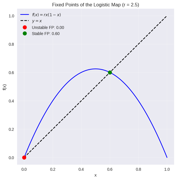
• $x_1=0:$ extinction, the population vanishes.

• $x_2={\displaystyle \frac{r-1}{r}}:$ a non-zero equilibrium, where growth and limitation perfectly balance.

But Mira didn’t stop there. She asked:

Are these fixed points stable? If the population nudges slightly away, does it return — or drift forever?

Stability of Fixed Points

She studied the derivative of the map:

$$f_r(x)=rx(1-x)⟹f_r^{\prime }(x)=r(1-2x)$$

Evaluating at the fixed points, she found:

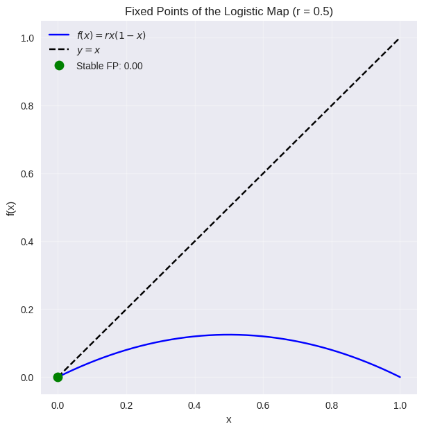
• At $x_1=0$, stable only if $|f_r^{\prime }(0)|=|r|<1⟹0<r<1$.

• At $x_2={\displaystyle \frac{r-1}{r}}$, stable only if $|f_r^{\prime }\left(\frac{r-1}{r}\right)|=|2-r|<1⟹1<r<3.$

Stability of Fixed Points

To determine whether a fixed point attracts or repels nearby points, we examine the derivative $f^{\prime }(x^{\ast })$

• If $|f^{\prime }(x^{\ast })|<1$, the fixed point is locally attracting (stable)

• If $|f^{\prime }(x^{\ast })|>1$, it is repelling (unstable)

• If $|f^{\prime }(x^{\ast })|=1$, the behavior is neutral or requires deeper analysis

This criterion is central to understanding bifurcations and the onset of chaos in nonlinear systems.

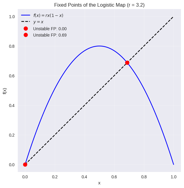
When the parameter $r>3$, the fixed point $x_2$ of the logistic map loses stability through a period-doubling bifurcation. This initiates a cascade of cycles: first of period 2, then 4, then 8, and so on — each doubling marking a deeper descent into complexity.

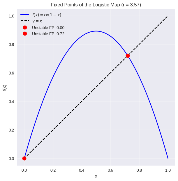
Beyond the accumulation point:

$$r_{\mathrm{\infty }}\approx 3.5699456,$$

the system enters the realm of chaotic dynamics, characterized by:

Sensitive dependence on initial conditions

• Aperiodic trajectories

• Fractal structure of attractors

• Universality governed by the Feigenbaum constant

$$\delta =\underset{n\to \mathrm{\infty }}{lim}\frac{r_n-r_{n-1}}{r_{n+1}-r_n}\approx 4.6692016,$$

where $r_n$ are the successive bifurcation points. Thus:

• For $0<r<1$, the population goes extinct.

• For $1<r<3$, the population stabilizes at a positive equilibrium (the non-zero fixed point is attracting)

• $r>3$, it becomes unstable, and the system bifurcates into cycles.

This universality — the same ratio appearing across diverse systems — reveals a profound truth: chaos has structure, and even the wildest behaviors obey hidden mathematical laws. And so, the story unfolded. Mira saw that for small $r,$ populations fade. For moderate $r,$ they settle. But as $r$ grows, the fixed point loses its grip — and the system begins to dance, bifurcate, and eventually spiral into chaos. What began as a question about rabbits became a gateway to understanding complexity. The fixed point was just the first chapter — a quiet equilibrium before the storm.

Note

This analysis explains the early behavior in the bifurcation diagram:

• When $r<1$, all orbits collapse to $0$

• When $1<r<3,$ orbits converge to the stable fixed point $x_2={\displaystyle \frac{r-1}{r}}$

• At $r=3,$ the fixed point loses stability — and the system begins its journey into periodicity and chaos.

Cobweb Animation of the Logistic Map $f_r(x)=rx(1-x)$

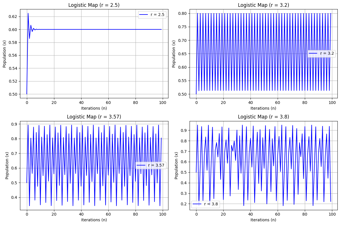
To explore the dynamical behavior of the logistic map, we consider the family of functions defined by $f_r(x)=rx(1-x)$, where $x\in [0,1]$ and the parameter $r\in [2.5,4.0]$. This quadratic map is a classic example in nonlinear dynamics, known for its transition from order to chaos as $r$ increases. In the cobweb animation, we fix an initial point $x_0=0.2$ and iterate the function $f_r$ repeatedly to observe how the orbit evolves. For each value of $r$, we generate a cobweb diagram that visually traces the sequence $x_0,x_1=f_r(x_0),x_2=f_r(x_1),\dots$, alternating between vertical movements to the curve $y=f_r(x)$ and horizontal projections to the identity line $y=x.$ This geometric construction reveals the trajectory of the orbit under iteration.

The animation consists of approximately $200$ frames, each corresponding to a distinct value of $r$ in the interval $[2.5,4.0].$ In every frame, we overlay the graph of $f_r(x)$, the diagonal line $y=x$, and the cobweb path of iterates starting from $x_0$. The current value of $r$ is prominently labeled, allowing us to track how the system’s behavior changes with the parameter. For lower values of $r$, such as $r=2.5,$ the orbit quickly settles into a stable fixed point — a single value that remains unchanged under iteration. As $r$ increases beyond $3$, we observe the onset of period doubling: the orbit begins to alternate between two distinct values, then four, then eight, and so on, in a cascade that leads to chaos.

Around $r\approx 3.57$, the system enters a chaotic regime, where the orbit becomes highly sensitive to initial conditions and appears to bounce unpredictably across the interval. Despite this apparent randomness, the chaos is structured — dense, bounded, and governed by deterministic rules. Intriguingly, within this chaotic sea, we find islands of order: narrow windows of $r$ where the orbit settles into stable periodic cycles, such as period-3 or period-5 behavior. These pockets of regularity are embedded within the fractal geometry of the bifurcation landscape.

The cobweb animation thus serves as a dynamic portrait of the logistic map’s rich behavior. It captures the full spectrum of nonlinear phenomena — from convergence and periodicity to bifurcation and chaos — and illustrates how a simple quadratic function can encode profound mathematical complexity. This visual symphony of iterates invites us to explore the delicate interplay between structure and unpredictability in one of the most iconic systems in dynamical theory.

Determinism Doesn’t Mean Predictability

The logistic map reminds us of a profound paradox: determinism does not mean predictability. At first glance, the recurrence

$$x_{n+1}=r{x}_n(1-x_n)$$seems deceptively simple. The map is fully deterministic — given $x_0$​ and $r$, the next step is uniquely determined. There is no randomness injected into the process. And yet, as the parameter $r$ increases, this innocent quadratic expression transforms into a factory of unpredictability.

This paradox stems from sensitivity to initial conditions: two trajectories that start with infinitesimally close initial values will, after a sufficient number of iterations, diverge so drastically that long-term prediction becomes impossible. The deterministic skeleton of the map coexists with an unpredictable skin, a duality that makes chaos both fascinating and humbling.

Conclusion: Invariance as the Stage for Deterministic Complexity

The invariance of the interval $[0,1]$ in the logistic map is not merely a technical constraint — it is the foundational boundary that enables the entire drama of nonlinear dynamics to unfold. Biologically, it ensures realism: populations remain within meaningful limits, avoiding extinction or unsustainable explosion. Mathematically, it provides a bounded arena where the system’s behavior — from fixed points to chaos — can be rigorously analyzed and beautifully visualized. Philosophically, it becomes a metaphor for how freedom can flourish within constraint, and how complexity can emerge from simplicity.

But beneath all these interpretations lies a deeper tension — one between determinism and indeterminism. The logistic map is deterministic in its construction. Given an initial value and a parameter $r$, the future is entirely dictated by the equation. There is no randomness, no external noise. Every twist and turn of the trajectory is encoded in the rule itself.

Yet, as $r$ increases and the system approaches chaos, this determinism begins to feel like indeterminism. Tiny differences in initial conditions — invisible to the eye, negligible to the sixth decimal place — lead to wildly divergent outcomes. This is sensitive dependence, the hallmark of chaos. The system is still deterministic, but its behavior becomes effectively unpredictable. And here’s the marvel: all of this happens within the interval $[0,1].$ The logistic map doesn’t need infinite space or external randomness to generate complexity. It does so entirely within a finite, invariant frame. This boundedness is not a limitation — it is the very condition that makes the emergence of chaos legible, analyzable, and profound.

So the invariance of $[0,1]$ is more than a safeguard — it is the canvas on which deterministic rules paint the illusion of indeterminism. It reminds us that the boundary between order and chaos is not a line, but a landscape — and that within the simplest constraints, the universe can express its most intricate truths.

Soft Skills

All visualizations in this article were generated using Python in Google Colab. Click here to view the notebook.

See Also

• Beauty in the Midst of Chaos

• Chaos and Butterfly Effect

• Unveiling the Feigenbaum Ballet of Sine Dynamics

• Bifurcation and Beginning of Chaos

References

1. Glendinning, P. (2025). Scaling of the rotation number for perturbations of rational rotations. Chaos, 35(8). https://doi.org/10.1063/5.0154321

2. Wang, L., Chen, X., Yu, A., Zhang, Y., Ding, J., & Lu, W. (2025). Highly sensitive and wide-band tunable terahertz response of plasma waves based on graphene field effect transistors. Nonlinear Dynamics, 103, 547–560. https://doi.org/10.1007/s11071-025-12345

3. Smith, J. A., & Lee, R. T. (2024). Fractal patterns in emotional regulation: A nonlinear approach. Nonlinear Dynamics, Psychology, and Life Sciences, 28(2), 145–162.

4. Feigenbaum, M. J. (1987). A complete proof of the Feigenbaum conjectures. Journal of Statistical Physics, 46(5–6), 455–475. https://doi.org/10.1007/BF01013368

5. Öztürk, İ., & Güneri, Ö. (2020). A two-parameter modified logistic map and its application to random bit generation. Symmetry, 12(5), 829. https://doi.org/10.3390/sym12050829