Unveiling the Feigenbaum Ballet of Sine Dynamics

Mapping Chaotic Elegance

Abstract

The Feigenbaum diagram stands as a visual testament to the intricate journey of period-doubling leading to chaos within dynamic systems, particularly underscored by the well-studied logistic map. However, our investigation takes an innovative turn towards the less-explored landscape of the sine map—a one-dimensional dynamical system endowed with the capacity to unveil complex bifurcation phenomena reminiscent of its logistic counterpart. In this study, we embark on an intellectual odyssey to delineate and comprehend the nuances of the Feigenbaum diagram when applied to the sine map. Contrary to the well-established narrative of the logistic map, the sine map introduces a unique cadence to the symphony of chaos, weaving a tapestry of bifurcation patterns that demand nuanced examination. The graphical representation becomes a canvas on which the intricate interplay between system parameters and emergent chaotic behavior is painted. As we traverse this mathematical terrain, the allure of chaos and order converges in a captivating dance, revealing underlying principles that echo across the diverse spectrum of nonlinear maps. Our exploration delves beyond mere comparison, seeking to uncover the universal essence that unites these seemingly disparate mathematical entities.

1 Objective

• Modeling the Pitchfork bifurcation of Sine Map.

• Constructing Feigenbaum Diagram in Sine Map.

• Numerical verification of Feigenbaum constant

  \[ \delta = \frac{{\mu}_n - {\mu}_{n+1}}{\mu_{n+1}-\mu_n} = 4.699\ldots \]

2 Methodology

The sine map is defined by the recurrence relation:

\[ x_{n+1} = \mu \sin(\pi x_n) \; \; \text{where};\ x_0, \mu \in [0,1] \]

where \(x_n\)​ is the state of the system at time \(n\), \(\mu\) is a parameter.

To create an empirical Feigenbaum diagram for the sine map, you would typically follow these steps:

1. Choose a Range of \(\mu\): Select a range of values for the parameter \(\mu\). This range should include values where interesting bifurcation behavior occurs.

2. Initialize \(x_0\)​: Choose an initial condition \(x_0\).

3. Iterate the Map: For each value of \(\mu\) in your chosen range, iterate the map equation for a certain number of iterations, discarding an initial transient to allow the system to reach its attractor.

4. Plot the Results: For each \(r\) plot the values of \(x_n\) after the transient has passed. This will give you a bifurcation diagram showing how the system’s behavior changes with varying \(\mu\).

5. Repeat: If needed, refine your results by increasing the number of iterations or changing the range of \(\mu\).

It’s important to note that while the logistic map has a well-known Feigenbaum constant (about \(4.669\)), the sine map may not have a universal constant. The Feigenbaum diagram for the sine map will still exhibit bifurcation cascades, but the exact values may differ. The process of creating an empirical Feigenbaum diagram for the sine map is similar to that of other maps. It involves systematically exploring the parameter space and observing the bifurcation patterns that emerge as the parameter is varied.

# Function to iterate the sine map
sine_map_iteration <- function(x, mu) {
  return(mu * sin(pi * x))
}

# Function to generate the bifurcation diagram
generate_bifurcation_diagram <- function(mu_values, iterations, transient) {
  # Create a matrix to store the bifurcation diagram
  bifurcation_diagram <- matrix(nrow = iterations - transient, ncol = length(mu_values))
  
  # Iterate through mu values
  for (i in seq_along(mu_values)) {
    mu <- mu_values[i]
    x <- runif(1)  # Initial condition (you can experiment with different initial conditions)
    
    # Iterate the sine map
    for (j in 1:iterations) {
      x <- sine_map_iteration(x, mu)
      if (j > transient) {
        bifurcation_diagram[j - transient, i] <- x
      }
    }
  }
  
  # Transpose the matrix before plotting
  bifurcation_diagram <- t(bifurcation_diagram)
  
  # Plot the bifurcation diagram
  matplot(mu_values, bifurcation_diagram, pch = ".", col = "black", cex = 0.1,
          xlab = expression(mu), ylab = expression(x[n]))
}

# Set parameters
mu_values <- seq(0, 3, by = 0.005)  # Range of mu values
iterations <- 1200  # Number of iterations per mu value
transient <- 200  # Transient iterations to discard

# Generate and plot the bifurcation diagram
generate_bifurcation_diagram(mu_values, iterations, transient)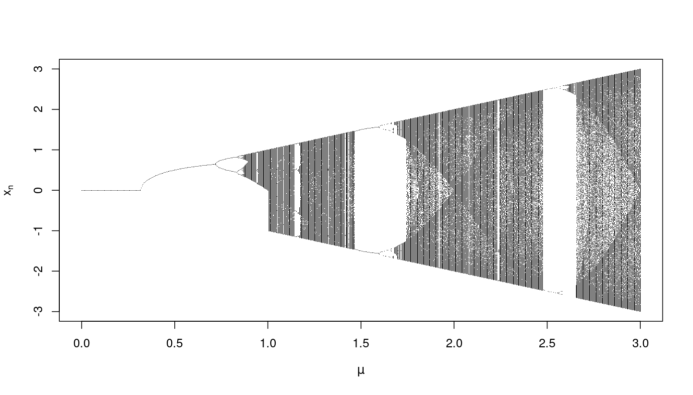

Conclusion

This study not only contributes to the understanding of the sine map’s bifurcation behavior but also prompts broader reflections on the applicability and transferability of bifurcation concepts across different dynamical systems. The narrative woven by the sine map, as illuminated through the Feigenbaum diagram, serves as an intellectual gateway into the profound interconnections between chaos theory and nonlinear dynamics. In doing so, this study enriches the discourse surrounding bifurcation phenomena and their manifestations in diverse mathematical landscapes.

See Also

• Bifurcation and The Beginning of Chaos

• Chaos and Butterfly Effect

Footnotes

• The Feigenbaum Constant (4.669) – Numberphile, retrieved 7 February 2023

• Feigenbaum, M. J. (1976). “Universality in complex discrete dynamics” (PDF). Los Alamos Theoretical Division Annual Report 1975–1976.

References

1. Briggs, Keith (July 1991). “A Precise Calculation of the Feigenbaum Constants” (PDF). Mathematics of Computation. 57 (195): 435–439. Bibcode:1991MaCom..57..435B. doi:10.1090/S0025-5718-1991-1079009-6.

2. Briggs, Keith (1997). Feigenbaum scaling in discrete dynamical systems (PDF) (PhD thesis). University of Melbourne.

3. Broadhurst, David (22 March 1999). “Feigenbaum constants to 1018 decimal places”.