Algorithmic Elegance: Fractal Symphonies in R
Unveiling Chaotic Elegance
At first, it will look pretty random but soon a familiar form emerges. The trajectories that began on the edges seem to speed off in random directions. But all those that began within a certain space end up in the attractor. It might seem like their starting positions no longer matter, but once they reach the attractor, their trajectories diverge, each following its path indefinitely, and they never cross. So, the small differences in their start positions lead to increasingly different futures.
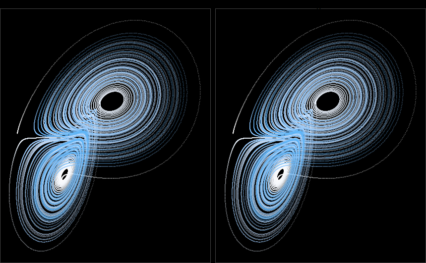

This is the poster child of chaos theory and is sometimes almost synonymous with the butterfly effect or the field of chaos theory itself. It even looks like a butterfly.
Trajectories are just curves, so they should be 1-dimensional. But how come no matter how much you zoom in on this attractor, you can always find more and more trajectories everywhere?
This is the reason that this attractor is said to have a non-integer dimension. It’s made up of infinitely long curves in a finite space, which are so detailed that they start to partially fill up a higher dimension. It’s not 1 dimensional, 2 dimensional, or 3 dimensional - it’s dimension is somewhere in between. As a result of this non-integer dimension and detail of arbitrarily small scales, the set of points in the Lorenz attractor is a fractal space, and that’s why it’s a strange attractor.
A strange attractor has a fractal structure. A fractal structure is a geometric shape that has a fractional dimension.
Bridging Science and Aesthetics
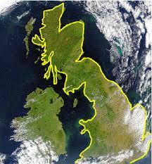
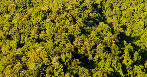
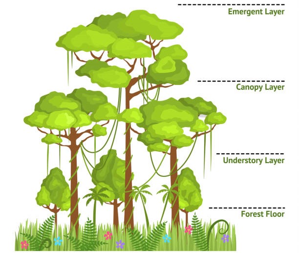
Chaos, present in everything from a drop of water to the galaxies in our universe, has long fascinated people from cultures around the world. The natural disorder present in the branches of trees, lightning, and coastlines, to name a few examples, may seem to be completely chaotic. However, self-similarity within these phenomena is much more organized than it appears. Repeating patterns in many natural objects and processes are known as fractals – figures that show self-similarity at different levels.
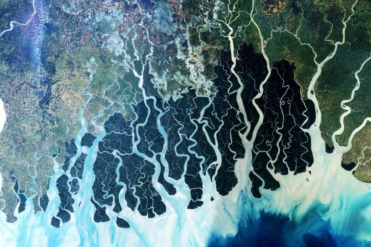

The Fascinating World of Natural Fractals
Fractals are patterns formed from what is known as chaotic equations. They exhibit self-similar patterns of complexity regardless of magnification. When divided into parts, they produce a nearly identical, reduced-sized copy of the whole. With fractals, infinite complexity is formed with relatively simple equations. By iterating or repeating these equations many times, random outputs create amazing patterns that are unique yet recognizable. However, most fractals in nature do not repeat forever. The repetition eventually breaks down in natural patterns, and they cease to be fractals. In many cases, fractal patterns are the most efficient way to deliver nutrient-harvested sunlight or form support structures for plants or animals.

Towards the Realm of Fractal
Self-Similarity & Fractals
Self-similarity, a fascinating property observed in nature, forms the cornerstone of Benoit Mandelbrot’s pioneering work in fractal geometry. This concept entails objects appearing identical regardless of the scale at which they are observed, offering profound insights into the intricate patterns found in natural phenomena. When looking around nature, you might have noticed intricate plants like these:
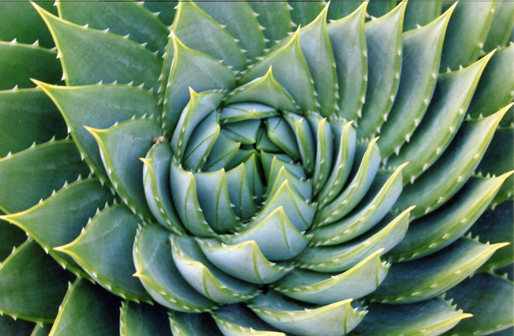

Initially, these appear like highly complex shapes – but when you look closer, you might notice that they both follow a relatively simple pattern: all the individual parts of the plants look the same as the entire plant, just smaller. The same pattern is repeated over and over again, at smaller scales. In mathematics, we call this property self-similarity, and shapes that have it are called fractals.
The Output
The Mystery
We were engaged in the exploration of random phenomena, and the intrigue surrounding these random occurrences lies in the game we were actively participating in. The revelation of this interesting aspect becomes apparent when we alter the system of equations in a specific manner.
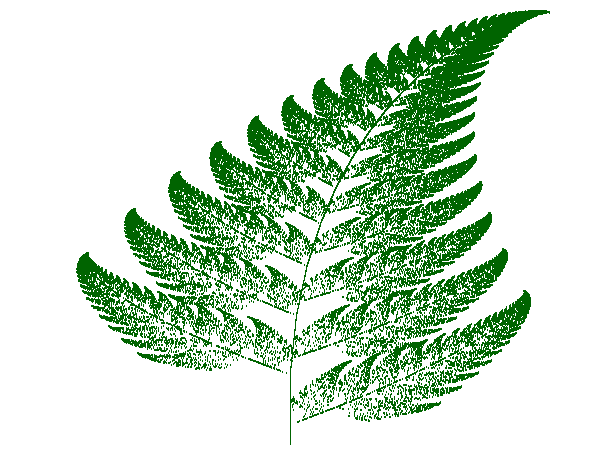
| A number appears in the dice | Where the particle moves |
|---|---|
| 1 | \((0,0.16y)\) |
| 2 | \((0.85x-0.04y,-0.04x+0.85y+1.6)\) |
| 3 | \((0.2x-0.26y,0.23x+0.22y+1.6)\) |
| 4 | \((-0.15x+0.28y,0.26x+0.24y+0.44)\) |
pBarnsleyFern <- function(fn, n, clr, ttl, psz=600) {
  cat(" *** START:", date(), "n=", n, "clr=", clr, "psz=", psz, "\n");
  cat(" *** File name -", fn, "\n");
  pf = paste0(fn,".png"); # pf - plot file name
  A1 <- matrix(c(0,0,0,0.16,0.85,-0.04,0.04,0.85,0.2,0.23,-0.26,0.22,-0.15,0.26,0.28,0.24), ncol=4, nrow=4, byrow=TRUE);
  A2 <- matrix(c(0,0,0,1.6,0,1.6,0,0.44), ncol=2, nrow=4, byrow=TRUE);
  P <- c(.01,.85,.07,.07);
  # Creating matrices M1 and M2.
  M1=vector("list", 4); M2 = vector("list", 4);
  for (i in 1:4) {
    M1[[i]] <- matrix(c(A1[i,1:4]), nrow=2);
    M2[[i]] <- matrix(c(A2[i, 1:2]), nrow=2);
  }
  x <- numeric(n); y <- numeric(n);
  x[1] <- y[1] <- 0;
  for (i in 1:(n-1)) {
    k <- sample(1:4, prob=P, size=1);
    M <- as.matrix(M1[[k]]);
    z <- M%*%c(x[i],y[i]) + M2[[k]];
    x[i+1] <- z[1]; y[i+1] <- z[2];
  }
  plot(x, y, main=ttl, axes=FALSE, xlab="", ylab="", col=clr, cex=0.1);
  # Writing png-file
  dev.copy(png, filename=pf,width=psz,height=psz);
  # Cleaning
  dev.off(); graphics.off();
  cat(" *** END:",date(),"\n");
}
## Executing:
pBarnsleyFern("BarnsleyFernR", 100000, "dark green", "Barnsley Fern Fractal", psz=600)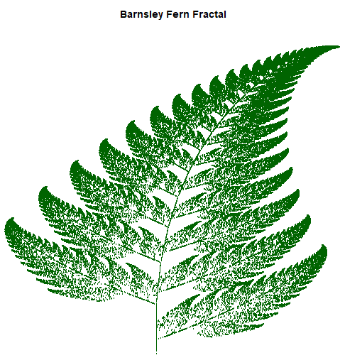
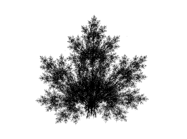
library(grid)
A=vector('list',4)
A[[1]]=matrix(c(0,0,0,0.18),nrow=2)
A[[2]]=matrix(c(0.85,-0.04,0.04,0.85),nrow=2)
A[[3]]=matrix(c(0.2,0.23,-0.26,0.22),nrow=2)
A[[4]]=matrix(c(-0.15,0.36,0.28,0.24),nrow=2)
b=vector('list',4)
b[[1]]=matrix(c(0,0))
b[[2]]=matrix(c(0,1.6))
b[[3]]=matrix(c(0,1.6))
b[[4]]=matrix(c(0,0.54))
n <- 500000
x <- numeric(n)
y <- numeric(n)
x[1] <- y[1] <- 0
for (i in 1:(n-1)) {
trans <- sample(1:4, prob=c(.02, .9, .09, .08), size=1)
xy <- A[[trans]]%*%c(x[i],y[i]) + b[[trans]]
x[i+1] <- xy[1]
y[i+1] <- xy[2]
}
plot(y,x,col= 'darkgreen',cex=0.1)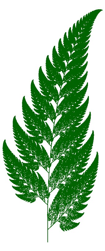
Canopy Chronicles
From Doodling to Natural Phenomena
Investigation into Iterative Drawing Algorithms
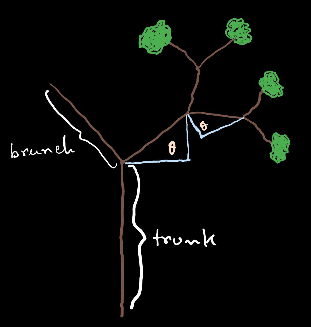
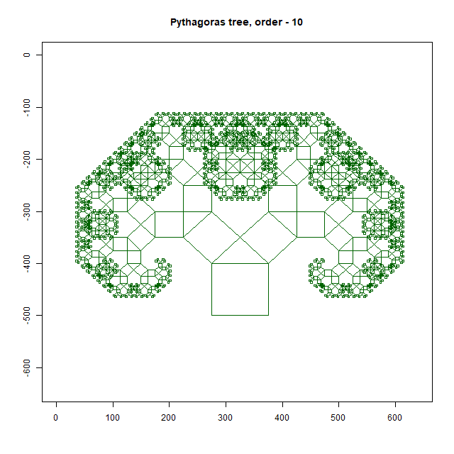
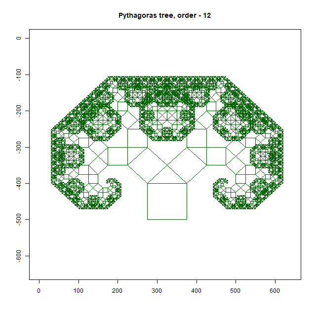
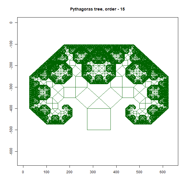
We’re investigating the implementation and application of iterative drawing algorithms, particularly focusing on recursive tree generation. The primary objective is to explore the rationale behind the development of code segments aimed at creating intricate tree-like structures through iterative processes.
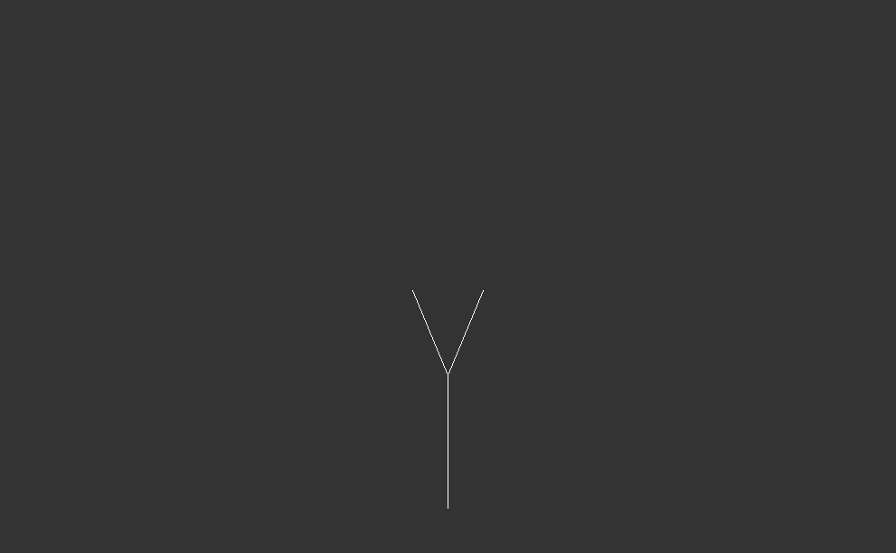
At the Beginning of the Iteration

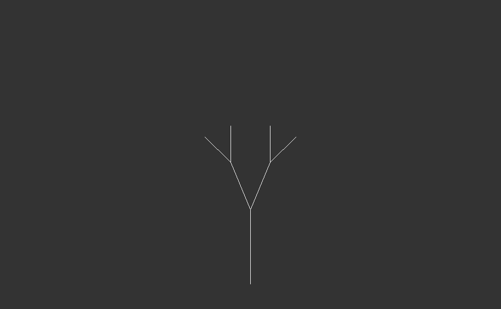


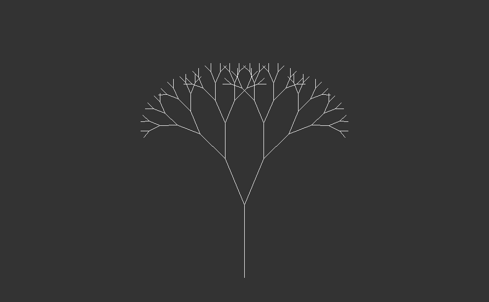
After Iteration 10
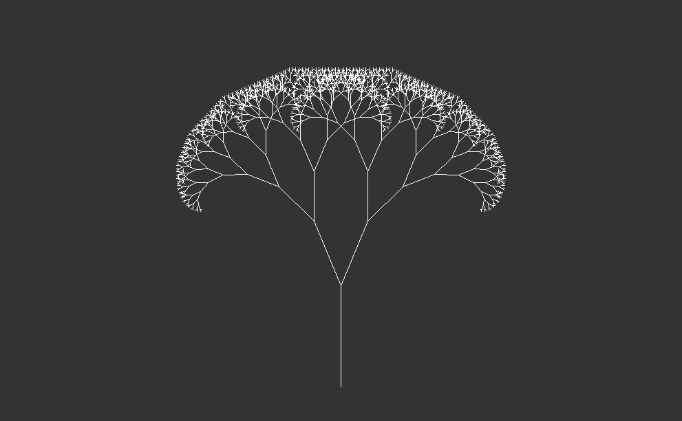
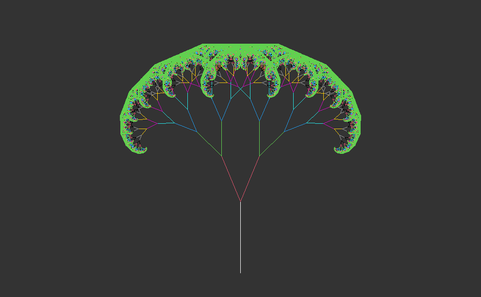
Nature’s Artistry
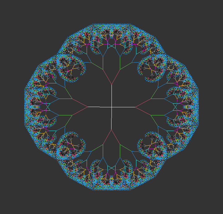
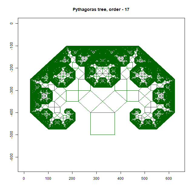
Pythagoras Tree
Sierpinski Triangle
Introduction
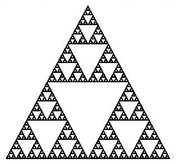
The Sierpinski triangle, named after the Polish mathematician Wacław Sierpiński, is one of the most iconic geometric fractals. This fractal is formed through a recursive process of subdividing a triangle into smaller triangles and removing the central triangle at each iteration. The resulting pattern is characterized by intricate triangular shapes nested within one another, demonstrating the mesmerizing beauty of self-similarity.
Origin
At its core, the Sierpinski triangle is a self-similar fractal, comprised of an equilateral triangle with smaller equilateral triangles recursively removed from its remaining area. This recursive removal process creates a fascinating visual effect, wherein the final shape consists of three identical copies of itself, each composed of even smaller copies of the entire triangle. This property allows for an endless zooming-in process, with patterns and shapes continuously repeating at ever-smaller scales.
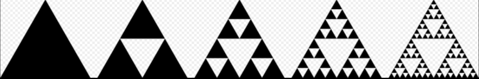
Construction
The construction of the Sierpinski triangle follows a systematic progression. Starting with a simple equilateral triangle, the first step involves removing the middle triangle, leaving behind three black triangles surrounding a central white triangle (iteration 1). This process is then repeated at a smaller scale, removing the middle third of each of the three remaining triangles, resulting in the second iteration with nine smaller black triangles. The number of smallest triangles triples with each iteration, yielding 27 triangles in the third iteration and 81 triangles in the fourth iteration. This tripling pattern continues indefinitely, and the number of triangles, denoted as \(T\), can be expressed as \(T=3^n\), where \(n\) represents the iteration level.
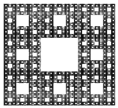
Sierpinski Carpet
Introduction
The Sierpinski Carpet, a captivating fractal pattern, was introduced by the Polish mathematician Wacław Sierpiński in 1916. This fractal, also known as the Sierpiński square or the Sierpiński sponge in three dimensions, exhibits intricate self-similarity and has captured the imagination of mathematicians, artists, and enthusiasts alike.
Origin
Wacław Sierpiński conceived the Sierpinski Carpet as a natural extension of his work on fractals, following his exploration of the Sierpinski triangle. The carpet’s inception marked a significant advancement in the understanding of fractal geometry and its applications across diverse fields.
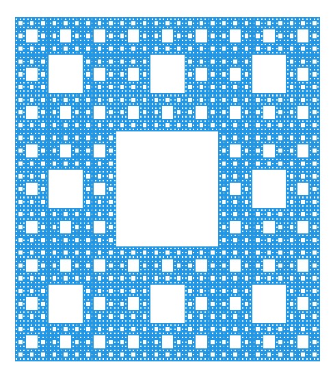
Construction
The construction of the Sierpinski Carpet follows a straightforward iterative process that yields strikingly complex results. Begin with a square divided into nine equal smaller squares arranged in a 3x3 grid. Remove the central square, leaving behind eight smaller squares. Repeat this process for each remaining square indefinitely. Through this recursive procedure, the Sierpinski Carpet emerges—a geometric wonder characterized by an infinitely repeating pattern of voids within a larger square.
The construction of the Sierpinski Carpet exemplifies the recursive nature of fractals, where simple rules repeated over and over again produce intricate and mesmerizing patterns. Despite its seemingly straightforward construction, the Sierpinski Carpet possesses remarkable properties, such as infinite perimeter and zero area, challenging conventional notions of geometry and dimensionality.
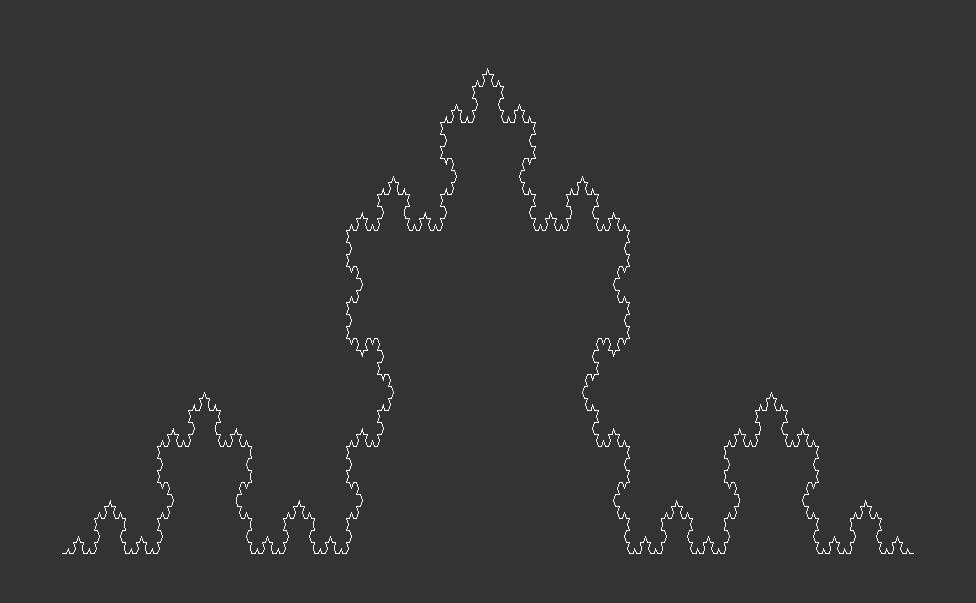
The Koch Snowflake
Introduction
In the realm of mathematical beauty, few patterns captivate the imagination quite like the Koch snowflake. This intricate fractal, named after the Swedish mathematician Helge von Koch, showcases the mesmerizing synergy between simplicity and complexity found in nature’s design. As we embark on our journey to unravel the secrets of this geometric wonder, we delve into its origins, construction, and significance in both mathematics and the natural world.
Origins
The story of the Koch snowflake begins in the early 20th century when Helge von Koch introduced the concept as a means to explore the notion of infinite perimeter within a finite area. In 1904, Koch presented his groundbreaking paper, “On a Continuous Curve Without Tangents, Constructible from Elementary Geometry,” unveiling this remarkable fractal.
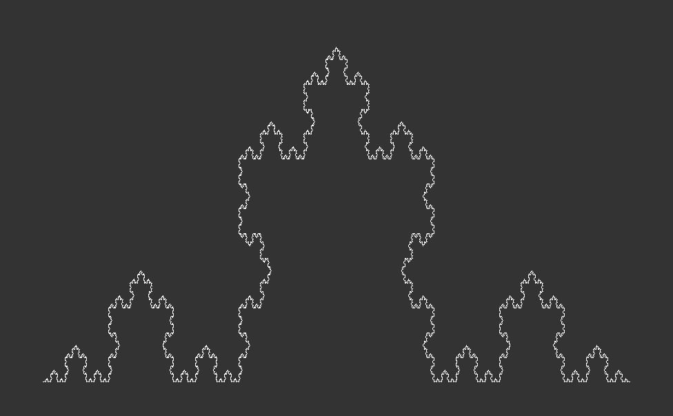
Construction
At its core, the Koch snowflake emerges from a deceptively simple iterative process. Start with an equilateral triangle, then replace the middle third of each line segment with two segments of equal length, forming a smaller equilateral triangle. Repeat this process infinitely for each remaining line segment, and behold—the Koch snowflake emerges in all its intricate glory. Despite its seemingly straightforward construction, the Koch snowflake possesses an infinite perimeter, yet encloses a finite area—an astounding paradox that showcases the beauty of fractal geometry.