“Mathematics possesses not only truth but supreme beauty—a beauty cold and austere, like that of sculpture.” – Bertrand Russell
Mathematics is replete with sequences that fascinate, challenge, and inspire. Among these is Recamán’s sequence, a non-traditional and intriguing sequence defined by a simple set of rules yet exhibiting complex and often surprising behaviour. Named after its creator, Colombian mathematician Bernardo Recamán Santos, this sequence offers a rich ground for exploration in number theory and recreational mathematics.
Definition and Construction
Recamán’s sequence \(\{a\}_{n\ge1}\) is defined as,
\[
\begin{equation} a_n= \begin{cases} 0, & \text{if } n=0\\ a_{n-1}-n, & \text{if } a_{n-1}-n >0\ \text{and is not already in the sequence} \\ a_{n-1}+n, & \text{otherwise } \end{cases}\end{equation}
\]
This definition can be summarized in the form of an algorithm:
Initial step: \(a_0 = 0\)
Recursive step: For \(n>0:\)
If \(a_{n−1}−n>0\ \text{and}\)\(a_{n−1}−n\ \text{has not been used before, then}\)\(a_n=a_{n−1}−n\)
Otherwise, \(a_n=a_{n−1}+n\)
To better understand the construction, let’s compute the first few terms of Recamán’s sequence:
\(a_0 =0\)
\(a_1 = 0+1 =1\)
\(a_2 = 1-2 =-1\ \text{(not allowed since it is negative, so)}\ a_2 = 1+2=3\)
\(a_3 = 3-3 = 0\ \text{(already in the sequence,so)}\ a_3 =3+3 =6\)
\(a_4 = 6-4 =2\)
\(a_5 = 2-5 =-3\ \text{(not allowed since it is negative, so)}\ a_5 =2+5=7\)
\(a_6 = 7-6 = 1\text{(already in the sequence,so)}\ a_6 =7+6 =13\)
Continuing in this manner, the sequence begins as, \(0, 1, 3, 6, 2, 7, 13, 20, 12, 21, 11, 22, 10,\ldots\) This sequence is known for its interesting properties, such as the seemingly chaotic pattern of values and the fact that it often revisits the same values in different steps.
Properties and Patterns
Recamán’s sequence is known for its unpredictable and non-repetitive nature. Despite the straightforward rule governing its construction, the sequence does not follow a simple or easily discernible pattern. Some of its notable properties include:
Non-repetition: Each number in the sequence is unique, emphasizing the condition that no number should repeat.
Oscillatory behavior: The sequence oscillates, moving both forwards and backwards, but always progressing to larger values overall.
Density and Growth: The sequence grows indefinitely but with irregular gaps. As \(n\) increases, the differences between consecutive terms can become very large.
Visualization
One of the most captivating ways to understand Recamán’s sequence is through visualization. One can observe the dynamic and seemingly chaotic nature of the sequence by plotting the sequence, either on a number line or in more artistic forms such as arcs connecting consecutive terms. This visual approach often highlights the interplay between the sequence’s forward and backward movements, creating a visually appealing pattern.
Code
funcionSecuenciaRecaman1<-function(numero) { x<-vector() y<-vector() z<-0 i <-1while(i <= numero) { x[i] <- zif(i ==1){ y[i] <- z } else {if(y[i-1] - x[i] >0&is.na(match(y[i-1] - x[i],y))) { y[i] <- y[i-1] - x[i] } else { y[i] <- y[i-1] + x[i] } } z<- z+1 i = i+1 }return(cbind(x,y)) }funcionSecuenciaRecaman1(25)plottingChallenge<-function(numeral){#Recaman Sequence: (only retrieving values)laSecuencia <-funcionSecuenciaRecaman1(numeral)[,2]#declarandoVectoresNecesariospuntosEnx <-vector()puntosEny <-vector()ciclo <-vector()degrees <-c(1:179) #to simulate semi-circle we will need degrees from 1 : 179numeral2 <- numeral -1#Comienza el Ciclofor(i in1:numeral2){##These are the edges of the semi-circle (diameter of circle) x1<- laSecuencia[i] x2<- laSecuencia[i+1]##Evaluating whether semi-circle will curve upwards or downwards if(i%%2==0){curvaturaHaciaArriba <-1} else {curvaturaHaciaArriba <--1} radio <-abs(x2 - x1)/2#radius of circleif(x2>x1){puntoMedio <- x1+radio}else{puntoMedio <- x2+radio } alturas<-sin(degrees*pi/180)*radio*curvaturaHaciaArriba #all heights distancias <-cos(degrees*pi/180)*radio #all lengthsif(x2>x1){distancias1 <-sort(distancias,decreasing = F) } else {distancias1 <- distancias} puntosEnx <-c(puntosEnx,x1,distancias1 + puntoMedio,x2) puntosEny <-c(puntosEny,0,alturas,0)}matriz<-cbind(puntosEnx,puntosEny)matrizUnica<-unique(matriz)par(bg="black")plot(matrizUnica[,1],matrizUnica[,2], type ="l", main ="Secuencia de Recaman", xlab ="Seq. Recaman", ylab ="",col="white", #color del grafico#col.axis = "white", #estos son los numeritos,col.axis ="yellow", #titulos de los axiscex.lab =1 )points( tail(matrizUnica[,1],1), tail(matrizUnica[,2],1), pch =11, col ="yellow" )title("Recaman Sequence", col.main ="white")}plottingChallenge(50)plottingChallenge(100)plottingChallenge(150)plottingChallenge(200)plottingChallenge(500)plottingChallenge(1000)
R Code Breakdown
funcionSecuenciaRecaman1 Function
This function generates Recamán’s sequence up to a specified number of terms (numero).
funcionSecuenciaRecaman1 <-function(numero) { x <-vector() # Initialize vector x to store intermediate values y <-vector() # Initialize vector y to store Recamán's sequence values z <-0# Start with z = 0 (first term of the sequence) i <-1# Start with i = 1 (first iteration)while (i <= numero) { # Loop until i exceeds the specified number x[i] <- z # Assign the current value of z to x[i]if (i ==1) { # Special case for the first element y[i] <- z # Assign the current value of z to y[i] } else {# Check if y[i-1] - x[i] is positive and not already in yif (y[i-1] - x[i] >0&is.na(match(y[i-1] - x[i], y))) { y[i] <- y[i-1] - x[i] # Subtract x[i] from y[i-1] if condition is met } else { y[i] <- y[i-1] + x[i] # Otherwise, add x[i] to y[i-1] } } z <- z +1# Increment z for the next iteration i <- i +1# Increment i for the next iteration }return(cbind(x, y)) # Return a matrix with columns x and y}
Explanation:
Initialization:
x and y are empty vectors to store intermediate and sequence values.
z is initialized to 0, representing the first term of the sequence.
i is the loop counter starting from 1.
Loop (while (i <= numero)):
The loop runs until i exceeds the input numero.
In each iteration, x[i] is set to the current value of z.
For i = 1, y[i] is set to z directly.
For i > 1, the code checks if y[i-1] - x[i] is positive and not already in y. If true, it sets y[i] to y[i-1] - x[i]; otherwise, it sets y[i] to y[i-1] + x[i].
z and i are incremented in each iteration.
Return:
The function returns a matrix combining x and y.
plottingChallenge Function
This function generates a plot of Recamán’s sequence, visualizing the arcs between sequence values.
plottingChallenge <-function(numeral) {# Recamán Sequence: (only retrieving values) laSecuencia <-funcionSecuenciaRecaman1(numeral)[,2] # Get y values from the sequence# Declaring necessary vectors puntosEnx <-vector() # X coordinates for plotting puntosEny <-vector() # Y coordinates for plotting degrees <-c(1:179) # Degrees for semi-circle (from 1 to 179) numeral2 <- numeral -1# Begin the cyclefor (i in1:numeral2) {# These are the edges of the semi-circle (diameter of circle) x1 <- laSecuencia[i] x2 <- laSecuencia[i +1]# Ensure x1 and x2 are not NAif (is.na(x1) |is.na(x2)) {next }# Evaluating whether semi-circle will curve upwards or downwardsif (i %%2==0) { curvaturaHaciaArriba <-1 } else { curvaturaHaciaArriba <--1 } radio <-abs(x2 - x1) /2# Radius of circleif (x2 > x1) { puntoMedio <- x1 + radio } else { puntoMedio <- x2 + radio } alturas <-sin(degrees * pi /180) * radio * curvaturaHaciaArriba # All heights distancias <-cos(degrees * pi /180) * radio # All lengthsif (x2 > x1) { distancias1 <-sort(distancias, decreasing =FALSE) } else { distancias1 <- distancias } puntosEnx <-c(puntosEnx, x1, distancias1 + puntoMedio, x2) puntosEny <-c(puntosEny, 0, alturas, 0) } matriz <-cbind(puntosEnx, puntosEny) matrizUnica <-unique(matriz)par(bg ="black")plot(matrizUnica[,1], matrizUnica[,2], type ="l", main ="Secuencia de Recaman", xlab ="Seq. Recaman", ylab ="",col ="white", # Color of the plotcol.axis ="yellow", # Color of axis labelscex.lab =1 )points(tail(matrizUnica[,1], 1), tail(matrizUnica[,2], 1), pch =11, col ="yellow")title("Recaman Sequence", col.main ="white")}
Explanation:
Input Parameter: numeral specifies the number of terms to plot.
Sequence Generation: funcionSecuenciaRecaman1(numeral) generates the sequence, and [,2] retrieves the y-values.
Initialize Vectors:
puntosEnx and puntosEny store x and y coordinates for plotting.
degrees is a sequence from 1 to 179, representing angles for semi-circle calculations.
numeral2 is numeral - 1, representing the number of arcs.
Loop (for (i in 1:numeral2)):
Loop through each pair of terms to calculate the coordinates of arcs.
x1 and x2 are the consecutive terms in the sequence.
NA Check: Skip if either x1 or x2 is NA.
Direction of Arc: Determine whether the arc curves upwards or downwards based on the parity of i.
Radius and Midpoint Calculation: Calculate the radius and midpoint of the semi-circle.
Heights and Lengths Calculation: Calculate the y-coordinates (alturas) and x-coordinates (distancias) for the semi-circle.
Sorting Lengths: Ensure distancias are in the correct order based on the direction of the arc.
Store Coordinates: Append calculated coordinates to puntosEnx and puntosEny.
Plotting:
Combine puntosEnx and puntosEny into a matrix (matriz).
Remove duplicate points to get matrizUnica.
Set plot background to black and plot the sequence with white lines.
Highlight the final point in yellow.
Add title to the plot.
Running the Code
To visualize the Recamán sequence, you can call the plottingChallenge function with the desired number of terms. For example:
plottingChallenge(100)
This will generate a plot showing the first 100 terms of Recamán’s sequence with arcs connecting the terms. The visualization helps to see the fascinating pattern that emerges from this simple rule, demonstrating how mathematical sequences can often yield surprising and intricate structures.
Recamán’s Sequence with tidyverse()
This code is notable for its use of modern R packages and functions to generate and visualize Recamán’s sequence. It leverages the tidyverse package, particularly dplyr and ggplot2, to create a clean and effective visualization. Let’s break down the code to highlight its special features.
Code
library(tidyverse)# Generate the first n elements of the Recaman's sequenceget_recaman <-function(n) { recaman_seq <-numeric(n)for (i in1:length(recaman_seq)) { candidate <- recaman_seq[i] - iif (candidate >0&!(candidate %in% recaman_seq)) { recaman_seq[i +1] <- candidate } else recaman_seq[i +1] <- recaman_seq[i] + i } recaman_seq <- recaman_seq[-length(recaman_seq)] recaman_seq}get_recaman(20)# Get semicircle pathsconstruct_arc <-function(start, stop, type) { r <-abs(start - stop) /2 x0 <-min(c(start, stop)) + r y0 <-0if (type =="up_forward") { theta <-seq(pi, 0, -0.01) } elseif (type =="up_backwards") { theta <-seq(0, pi, 0.01) } elseif (type =="down_forward") { theta <-seq(pi, 2* pi, 0.01) } elseif (type =="down_backwards") { theta <-seq(2* pi, pi, -0.01) } x <- r *cos(theta) + x0 y <- r *sin(theta) + y0 df <-data.frame(x, y)}# Plot the first n elements of the Recaman's sequenceplot_recaman <-function(n, size =1, alpha =0.8) { recaman_seq <-get_recaman(n) df <-data.frame(start = recaman_seq,stop =lead(recaman_seq),# Alternating position of the semicirclesside =rep_len(c("down", "up"), length(recaman_seq))) %>%mutate(direction =ifelse(stop - start >0, "forward", "backwards"),type =paste(side, direction, sep ="_")) %>%filter(!is.na(stop)) l <-Map(construct_arc, start = df$start, stop = df$stop, type = df$type) df2 <-do.call("rbind", l)ggplot(df2, aes(x, y)) +geom_path(alpha = alpha, size = size) +coord_fixed() +theme_void()}plot_recaman(100, size =2)plot_recaman(300, size =1)plot_recaman(500, size =0.5, alpha =0.8)plot_recaman(1000, size =0.5, alpha =0.8)plot_recaman(1500, size =0.5, alpha =0.8)plot_recaman(2000, size =0.5, alpha =0.8)# Do you like the drawing? Save it!#ggsave("Recamán's sequence.png", height=3, width=5, units='in', dpi=800)
Algorithmic Justification
Recamán’s Sequence Generation (get_recaman):
Initialization: Start with the first element of the sequence as \(0\).
Iterative Process: For each subsequent index i, compute a candidate value by subtracting i from the current value. If the candidate is positive and not already in the sequence, it is added. Otherwise, add i to the current value.
Mathematical Insight: This process ensures that the sequence generates unique values as much as possible, balancing between subtraction and addition to explore new values.
Semicircle Path Construction (construct_arc):
Radius Calculation: The radius is half the distance between two consecutive points in the sequence.
Theta Values: Use trigonometric functions to generate x and y coordinates for the semicircle based on the calculated radius and center.
Type of Curve: Alternate between upward and downward curves to create a visually appealing pattern.
Plotting the Sequence (plot_recaman):
Data Frame Creation: Create a data frame with start and stop points for each semicircle, and determine the type (up or down) and direction (forward or backward) of each curve.
Arc Construction: Use the construct_arc function to generate paths for each segment.
Visualization: Plot the semicircles using ggplot2, with customizable parameters for size and transparency to enhance visual appeal.
Key Features
Efficient Sequence Generation: The get_recaman function effectively generates Recamán’s sequence by leveraging vector operations and conditional checks.
Dynamic Path Construction: The construct_arc function calculates semicircle paths based on start and stop points, ensuring the correct curvature direction.
Elegant Visualization: ggplot2 is used for high-quality, customizable plots that highlight the unique pattern of Recamán’s sequence.
High-Resolution Output: The ability to save the plot as a high-resolution image makes it suitable for various uses, from academic publications to artistic displays.
This R code provides a robust method for generating and visualizing Recamán’s sequence, combining algorithmic efficiency with mathematical elegance. The use of semicircles to represent the sequence values not only illustrates the mathematical properties of the sequence but also creates visually captivating patterns.
S. Farrag and W. Alexan, “Secure 2D Image Steganography Using Recamán’s Sequence,” 2019 International Conference on Advanced Communication Technologies and Networking (CommNet), Rabat, Morocco, 2019, pp. 1-6. doi: 10.1109/COMMNET.2019.8742368
Source Code
---title: "Mathematical Curves in Action"subtitle: "Recamán's Sequence and R Graphics"author: "Abhirup Moitra"date: 2024-06-18format: html: code-fold: true code-tools: trueeditor: visualcategories: [Mathematics, R programming]image: recaman.png---::: {style="color: navy; font-size: 18px; font-family: Garamond; text-align: center; border-radius: 3px; background-image: linear-gradient(#C3E5E5, #F6F7FC);"}**"Mathematics possesses not only truth but supreme beauty—a beauty cold and austere, like that of sculpture." – Bertrand Russell**:::Mathematics is replete with sequences that fascinate, challenge, and inspire. Among these is Recamán's sequence, a non-traditional and intriguing sequence defined by a simple set of rules yet exhibiting complex and often surprising behaviour. Named after its creator, Colombian mathematician [**Bernardo Recamán Santos**](https://math.stackexchange.com/users/235016/bernardo-recam%C3%A1n-santos), this sequence offers a rich ground for exploration in number theory and recreational mathematics.# **Definition and Construction**Recamán's sequence $\{a\}_{n\ge1}$ is defined as,$$\begin{equation} a_n= \begin{cases} 0, & \text{if } n=0\\ a_{n-1}-n, & \text{if } a_{n-1}-n >0\ \text{and is not already in the sequence} \\ a_{n-1}+n, & \text{otherwise } \end{cases}\end{equation}$$This definition can be summarized in the form of an algorithm:- **Initial step**: $a_0 = 0$- **Recursive step**: For $n>0:$ - If $a_{n−1}−n>0\ \text{and}$ $a_{n−1}−n\ \text{has not been used before, then}$ $a_n=a_{n−1}−n$ - Otherwise, $a_n=a_{n−1}+n$To better understand the construction, let’s compute the first few terms of Recamán's sequence:- $a_0 =0$- $a_1 = 0+1 =1$- $a_2 = 1-2 =-1\ \text{(not allowed since it is negative, so)}\ a_2 = 1+2=3$- $a_3 = 3-3 = 0\ \text{(already in the sequence,so)}\ a_3 =3+3 =6$- $a_4 = 6-4 =2$- $a_5 = 2-5 =-3\ \text{(not allowed since it is negative, so)}\ a_5 =2+5=7$- $a_6 = 7-6 = 1\text{(already in the sequence,so)}\ a_6 =7+6 =13$Continuing in this manner, the sequence begins as, $0, 1, 3, 6, 2, 7, 13, 20, 12, 21, 11, 22, 10,\ldots$ This sequence is known for its interesting properties, such as the seemingly chaotic pattern of values and the fact that it often revisits the same values in different steps.# **Properties and Patterns**Recamán's sequence is known for its unpredictable and non-repetitive nature. Despite the straightforward rule governing its construction, the sequence does not follow a simple or easily discernible pattern. Some of its notable properties include:- **Non-repetition**: Each number in the sequence is unique, emphasizing the condition that no number should repeat.- **Oscillatory behavior**: The sequence oscillates, moving both forwards and backwards, but always progressing to larger values overall.- **Density and Growth**: The sequence grows indefinitely but with irregular gaps. As $n$ increases, the differences between consecutive terms can become very large.# VisualizationOne of the most captivating ways to understand Recamán's sequence is through visualization. One can observe the dynamic and seemingly chaotic nature of the sequence by plotting the sequence, either on a number line or in more artistic forms such as arcs connecting consecutive terms. This visual approach often highlights the interplay between the sequence's forward and backward movements, creating a visually appealing pattern.```{r,eval=FALSE,warning=FALSE,message=FALSE}funcionSecuenciaRecaman1<-function(numero) { x<- vector() y<- vector() z<-0 i <- 1 while(i <= numero) { x[i] <- z if(i == 1){ y[i] <- z } else { if(y[i-1] - x[i] > 0 & is.na(match(y[i-1] - x[i],y))) { y[i] <- y[i-1] - x[i] } else { y[i] <- y[i-1] + x[i] } } z<- z+1 i = i+1 } return(cbind(x,y)) }funcionSecuenciaRecaman1(25)plottingChallenge<-function(numeral){#Recaman Sequence: (only retrieving values)laSecuencia <-funcionSecuenciaRecaman1(numeral)[,2]#declarandoVectoresNecesariospuntosEnx <- vector()puntosEny <- vector()ciclo <- vector()degrees <- c(1:179) #to simulate semi-circle we will need degrees from 1 : 179numeral2 <- numeral - 1#Comienza el Ciclofor(i in 1:numeral2){ ##These are the edges of the semi-circle (diameter of circle) x1<- laSecuencia[i] x2<- laSecuencia[i+1] ##Evaluating whether semi-circle will curve upwards or downwards if(i%%2 == 0){curvaturaHaciaArriba <- 1} else {curvaturaHaciaArriba <- -1} radio <- abs(x2 - x1)/2 #radius of circle if(x2>x1){puntoMedio <- x1+radio}else{puntoMedio <- x2+radio } alturas<- sin(degrees*pi/180)*radio*curvaturaHaciaArriba #all heights distancias <- cos(degrees*pi/180)*radio #all lengths if(x2>x1){distancias1 <- sort(distancias,decreasing = F) } else {distancias1 <- distancias} puntosEnx <- c(puntosEnx,x1,distancias1 + puntoMedio,x2) puntosEny <- c(puntosEny,0,alturas,0)}matriz<-cbind(puntosEnx,puntosEny)matrizUnica<-unique(matriz)par(bg="black")plot(matrizUnica[,1],matrizUnica[,2], type = "l", main = "Secuencia de Recaman", xlab = "Seq. Recaman", ylab = "", col="white", #color del grafico #col.axis = "white", #estos son los numeritos, col.axis = "yellow", #titulos de los axis cex.lab = 1 )points( tail(matrizUnica[,1],1), tail(matrizUnica[,2],1), pch = 11, col = "yellow" )title("Recaman Sequence", col.main = "white")}plottingChallenge(50)plottingChallenge(100)plottingChallenge(150)plottingChallenge(200)plottingChallenge(500)plottingChallenge(1000)```::: {layout-nrow="2"}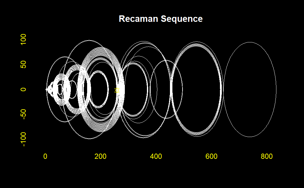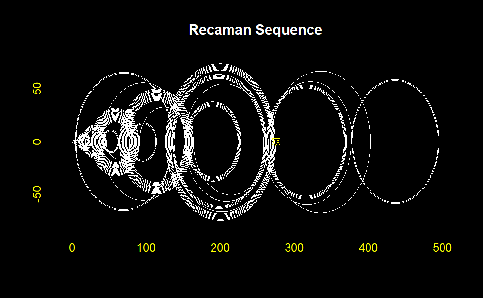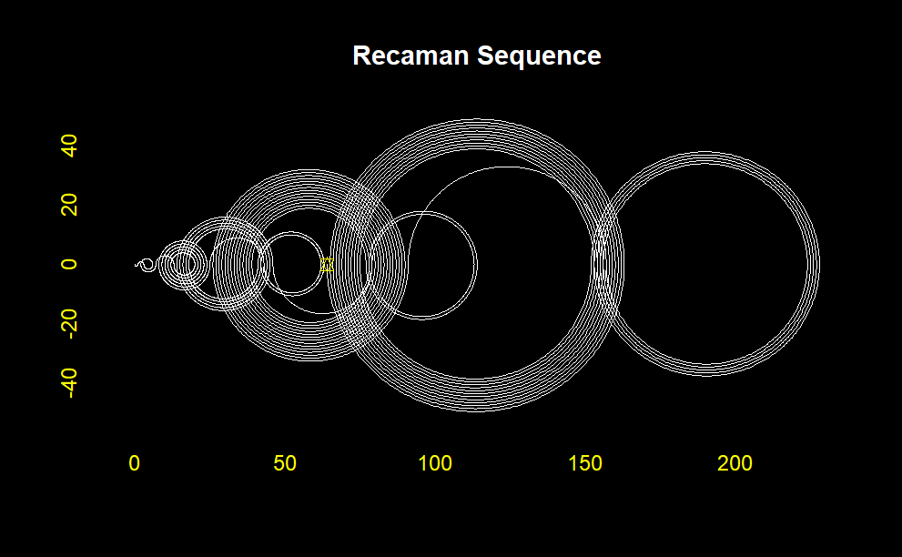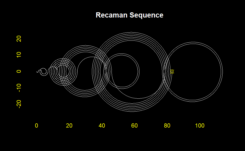:::::: {layout-ncol="2"}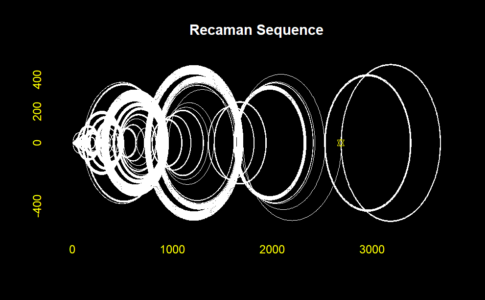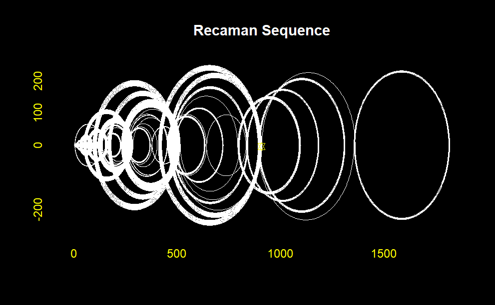:::## **R Code Breakdown**### **`funcionSecuenciaRecaman1` Function**This function generates Recamán's sequence up to a specified number of terms (`numero`).``` rfuncionSecuenciaRecaman1 <-function(numero) { x <-vector() # Initialize vector x to store intermediate values y <-vector() # Initialize vector y to store Recamán's sequence values z <-0# Start with z = 0 (first term of the sequence) i <-1# Start with i = 1 (first iteration)while (i <= numero) { # Loop until i exceeds the specified number x[i] <- z # Assign the current value of z to x[i]if (i ==1) { # Special case for the first element y[i] <- z # Assign the current value of z to y[i] } else {# Check if y[i-1] - x[i] is positive and not already in yif (y[i-1] - x[i] >0&is.na(match(y[i-1] - x[i], y))) { y[i] <- y[i-1] - x[i] # Subtract x[i] from y[i-1] if condition is met } else { y[i] <- y[i-1] + x[i] # Otherwise, add x[i] to y[i-1] } } z <- z +1# Increment z for the next iteration i <- i +1# Increment i for the next iteration }return(cbind(x, y)) # Return a matrix with columns x and y}```**Explanation**:- **Initialization**: - `x` and `y` are empty vectors to store intermediate and sequence values. - `z` is initialized to 0, representing the first term of the sequence. - `i` is the loop counter starting from 1.- **Loop (`while (i <= numero)`)**: - The loop runs until `i` exceeds the input `numero`. - In each iteration, `x[i]` is set to the current value of `z`. - For `i = 1`, `y[i]` is set to `z` directly. - For `i > 1`, the code checks if `y[i-1] - x[i]` is positive and not already in `y`. If true, it sets `y[i]` to `y[i-1] - x[i]`; otherwise, it sets `y[i]` to `y[i-1] + x[i]`. - `z` and `i` are incremented in each iteration.- **Return**: - The function returns a matrix combining `x` and `y`.### **`plottingChallenge` Function**This function generates a plot of Recamán's sequence, visualizing the arcs between sequence values.``` rplottingChallenge <-function(numeral) {# Recamán Sequence: (only retrieving values) laSecuencia <-funcionSecuenciaRecaman1(numeral)[,2] # Get y values from the sequence# Declaring necessary vectors puntosEnx <-vector() # X coordinates for plotting puntosEny <-vector() # Y coordinates for plotting degrees <-c(1:179) # Degrees for semi-circle (from 1 to 179) numeral2 <- numeral -1# Begin the cyclefor (i in1:numeral2) {# These are the edges of the semi-circle (diameter of circle) x1 <- laSecuencia[i] x2 <- laSecuencia[i +1]# Ensure x1 and x2 are not NAif (is.na(x1) |is.na(x2)) {next }# Evaluating whether semi-circle will curve upwards or downwardsif (i %%2==0) { curvaturaHaciaArriba <-1 } else { curvaturaHaciaArriba <--1 } radio <-abs(x2 - x1) /2# Radius of circleif (x2 > x1) { puntoMedio <- x1 + radio } else { puntoMedio <- x2 + radio } alturas <-sin(degrees * pi /180) * radio * curvaturaHaciaArriba # All heights distancias <-cos(degrees * pi /180) * radio # All lengthsif (x2 > x1) { distancias1 <-sort(distancias, decreasing =FALSE) } else { distancias1 <- distancias } puntosEnx <-c(puntosEnx, x1, distancias1 + puntoMedio, x2) puntosEny <-c(puntosEny, 0, alturas, 0) } matriz <-cbind(puntosEnx, puntosEny) matrizUnica <-unique(matriz)par(bg ="black")plot(matrizUnica[,1], matrizUnica[,2], type ="l", main ="Secuencia de Recaman", xlab ="Seq. Recaman", ylab ="",col ="white", # Color of the plotcol.axis ="yellow", # Color of axis labelscex.lab =1 )points(tail(matrizUnica[,1], 1), tail(matrizUnica[,2], 1), pch =11, col ="yellow")title("Recaman Sequence", col.main ="white")}```**Explanation**:- **Input Parameter**: `numeral` specifies the number of terms to plot.- **Sequence Generation**: `funcionSecuenciaRecaman1(numeral)` generates the sequence, and `[,2]` retrieves the y-values.- **Initialize Vectors**: - `puntosEnx` and `puntosEny` store x and y coordinates for plotting. - `degrees` is a sequence from 1 to 179, representing angles for semi-circle calculations. - `numeral2` is `numeral - 1`, representing the number of arcs.- **Loop (`for (i in 1:numeral2)`)**: - Loop through each pair of terms to calculate the coordinates of arcs. - `x1` and `x2` are the consecutive terms in the sequence. - **NA Check**: Skip if either `x1` or `x2` is NA. - **Direction of Arc**: Determine whether the arc curves upwards or downwards based on the parity of `i`. - **Radius and Midpoint Calculation**: Calculate the radius and midpoint of the semi-circle. - **Heights and Lengths Calculation**: Calculate the y-coordinates (`alturas`) and x-coordinates (`distancias`) for the semi-circle. - **Sorting Lengths**: Ensure `distancias` are in the correct order based on the direction of the arc. - **Store Coordinates**: Append calculated coordinates to `puntosEnx` and `puntosEny`.- **Plotting**: - Combine `puntosEnx` and `puntosEny` into a matrix (`matriz`). - Remove duplicate points to get `matrizUnica`. - Set plot background to black and plot the sequence with white lines. - Highlight the final point in yellow. - Add title to the plot.### **Running the Code**To visualize the Recamán sequence, you can call the `plottingChallenge` function with the desired number of terms. For example:``` rplottingChallenge(100)```This will generate a plot showing the first 100 terms of Recamán's sequence with arcs connecting the terms. The visualization helps to see the fascinating pattern that emerges from this simple rule, demonstrating how mathematical sequences can often yield surprising and intricate structures.# **Recamán's Sequence with `tidyverse()`**This code is notable for its use of modern R packages and functions to generate and visualize Recamán's sequence. It leverages the `tidyverse` package, particularly `dplyr` and `ggplot2`, to create a clean and effective visualization. Let's break down the code to highlight its special features.```{r,eval=FALSE, warning=FALSE, message=FALSE}library(tidyverse)# Generate the first n elements of the Recaman's sequenceget_recaman <- function(n) { recaman_seq <- numeric(n) for (i in 1:length(recaman_seq)) { candidate <- recaman_seq[i] - i if (candidate > 0 & !(candidate %in% recaman_seq)) { recaman_seq[i + 1] <- candidate } else recaman_seq[i + 1] <- recaman_seq[i] + i } recaman_seq <- recaman_seq[-length(recaman_seq)] recaman_seq}get_recaman(20)# Get semicircle pathsconstruct_arc <- function(start, stop, type) { r <- abs(start - stop) / 2 x0 <- min(c(start, stop)) + r y0 <- 0 if (type == "up_forward") { theta <- seq(pi, 0, -0.01) } else if (type == "up_backwards") { theta <- seq(0, pi, 0.01) } else if (type == "down_forward") { theta <- seq(pi, 2 * pi, 0.01) } else if (type == "down_backwards") { theta <- seq(2 * pi, pi, -0.01) } x <- r * cos(theta) + x0 y <- r * sin(theta) + y0 df <- data.frame(x, y)}# Plot the first n elements of the Recaman's sequenceplot_recaman <- function(n, size = 1, alpha = 0.8) { recaman_seq <- get_recaman(n) df <- data.frame(start = recaman_seq, stop = lead(recaman_seq), # Alternating position of the semicircles side = rep_len(c("down", "up"), length(recaman_seq))) %>% mutate(direction = ifelse(stop - start > 0, "forward", "backwards"), type = paste(side, direction, sep = "_")) %>% filter(!is.na(stop)) l <- Map(construct_arc, start = df$start, stop = df$stop, type = df$type) df2 <- do.call("rbind", l) ggplot(df2, aes(x, y)) + geom_path(alpha = alpha, size = size) + coord_fixed() + theme_void()}plot_recaman(100, size = 2)plot_recaman(300, size = 1)plot_recaman(500, size = 0.5, alpha = 0.8)plot_recaman(1000, size = 0.5, alpha = 0.8)plot_recaman(1500, size = 0.5, alpha = 0.8)plot_recaman(2000, size = 0.5, alpha = 0.8)# Do you like the drawing? Save it! #ggsave("Recamán's sequence.png", height=3, width=5, units='in', dpi=800)```::: {layout-nrow="2"}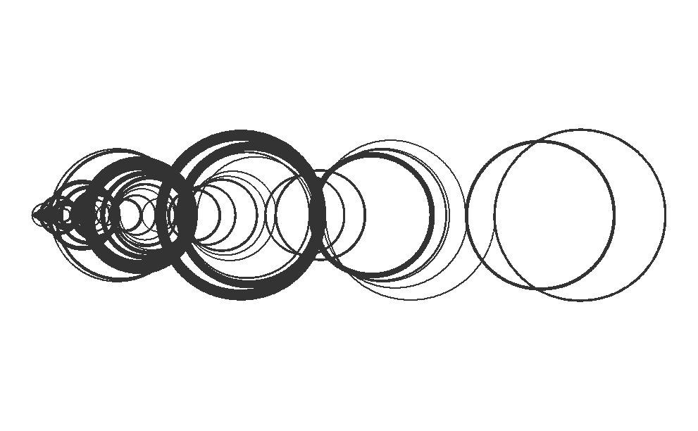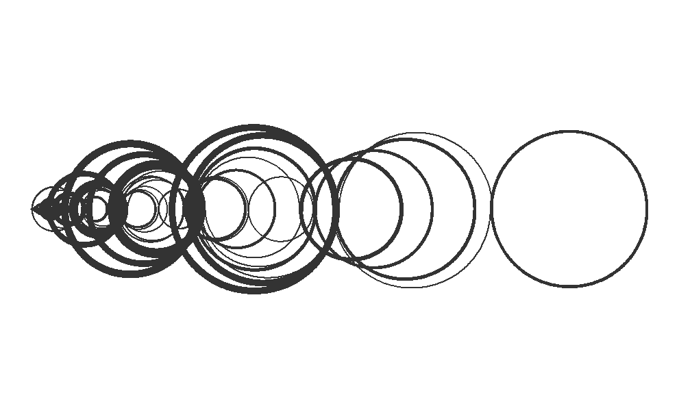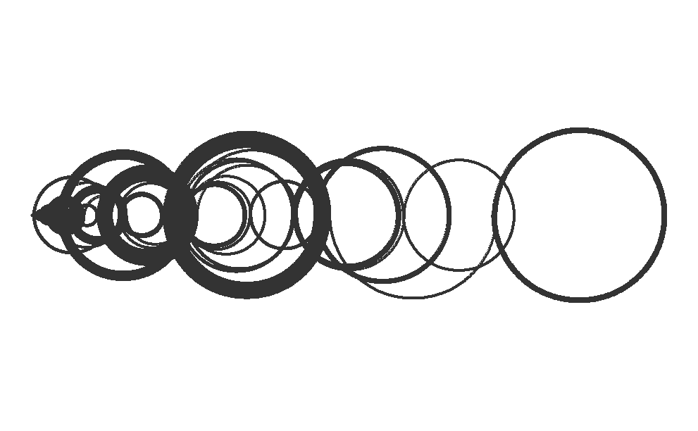:::::: {layout-ncol="2"}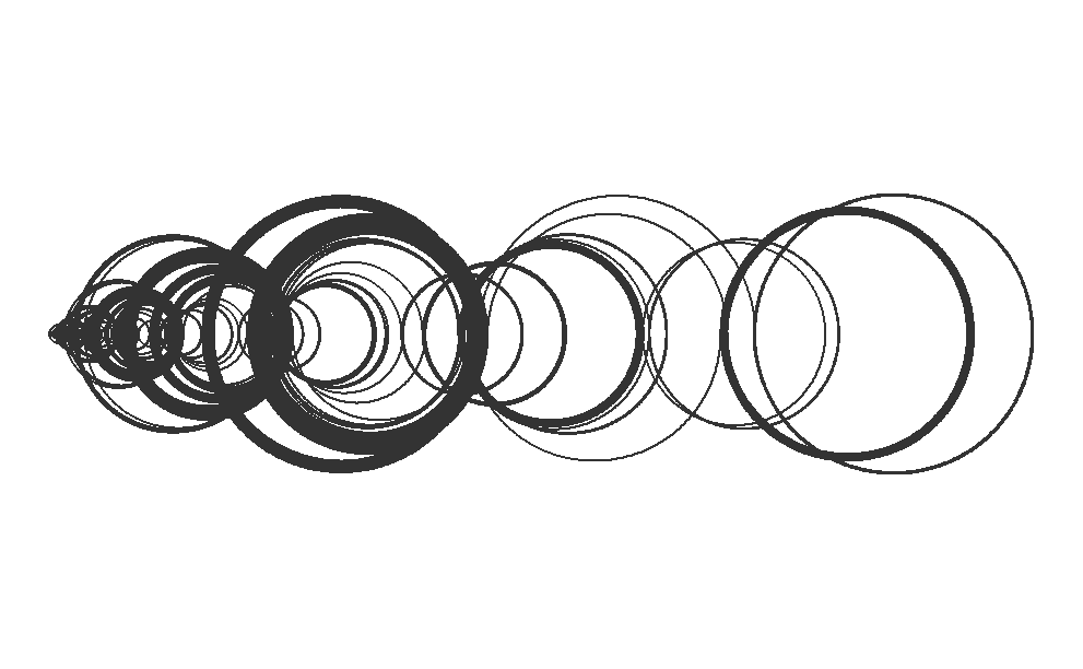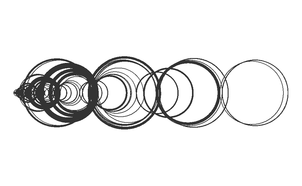:::## **Algorithmic Justification**1. **Recamán's Sequence Generation (`get_recaman`)**: - **Initialization**: Start with the first element of the sequence as $0$. - **Iterative Process**: For each subsequent index `i`, compute a candidate value by subtracting `i` from the current value. If the candidate is positive and not already in the sequence, it is added. Otherwise, add `i` to the current value. - **Mathematical Insight**: This process ensures that the sequence generates unique values as much as possible, balancing between subtraction and addition to explore new values.2. **Semicircle Path Construction (`construct_arc`)**: - **Radius Calculation**: The radius is half the distance between two consecutive points in the sequence. - **Theta Values**: Use trigonometric functions to generate x and y coordinates for the semicircle based on the calculated radius and center. - **Type of Curve**: Alternate between upward and downward curves to create a visually appealing pattern.3. **Plotting the Sequence (`plot_recaman`)**: - **Data Frame Creation**: Create a data frame with start and stop points for each semicircle, and determine the type (up or down) and direction (forward or backward) of each curve. - **Arc Construction**: Use the `construct_arc` function to generate paths for each segment. - **Visualization**: Plot the semicircles using `ggplot2`, with customizable parameters for size and transparency to enhance visual appeal.### Key Features1. **Efficient Sequence Generation**: The `get_recaman` function effectively generates Recamán's sequence by leveraging vector operations and conditional checks.2. **Dynamic Path Construction**: The `construct_arc` function calculates semicircle paths based on start and stop points, ensuring the correct curvature direction.3. **Elegant Visualization**: `ggplot2` is used for high-quality, customizable plots that highlight the unique pattern of Recamán's sequence.4. **High-Resolution Output**: The ability to save the plot as a high-resolution image makes it suitable for various uses, from academic publications to artistic displays.This R code provides a robust method for generating and visualizing Recamán's sequence, combining algorithmic efficiency with mathematical elegance. The use of semicircles to represent the sequence values not only illustrates the mathematical properties of the sequence but also creates visually captivating patterns.# **Motivation**{{< video https://youtu.be/FGC5TdIiT9U?si=8G8XS28JfdzNU3kQ >}}# **See Also**- [The Slightly Spooky Recamán Sequence. (June 14, 2018) Numberphile](https://www.youtube.com/watch?v=FGC5TdIiT9U) on [YouTube](https://en.wikipedia.org/wiki/YouTube_video_(identifier) "YouTube video (identifier)")- [The Recamán's sequence](http://rosettacode.org/wiki/Recaman%27s_sequence) at [Rosetta Code](https://en.wikipedia.org/wiki/Rosetta_Code "Rosetta Code")# **References**1. R.Ugalde, Laurence. ["Recamán sequence in Fōrmulæ programming language"](https://formulae.org/?example=Recam%C3%A1n%27s_sequence). *Fōrmulæ*. Retrieved July 26, 2021.2. S. Farrag and W. Alexan, "Secure 2D Image Steganography Using Recamán's Sequence," 2019 International Conference on Advanced Communication Technologies and Networking (CommNet), Rabat, Morocco, 2019, pp. 1-6. doi: 10.1109/COMMNET.2019.8742368{fig-align="center" width="484"}