this article delves into the intricate and astounding mathematics that underpins these seemingly simple designs. Through the lens of R programming, we will embark on a journey to uncover the hidden symmetries and patterns that adorn walls and fabrics around the world.
The Mathematics Behind Wallpaper Patterns
At its core, the study of wallpaper patterns is rooted in group theory and symmetry. These patterns can be classified into 17 distinct groups, each defined by a combination of translations, rotations, reflections, and glide reflections. The mathematical elegance of these symmetries not only provides a systematic way to create intricate designs but also reveals the underlying structure of the patterns we see in our everyday surroundings.
Bridging Art and Mathematics
The beauty of wallpaper patterns lies in their ability to transform simple geometric rules into complex and visually stunning artwork. By understanding the mathematical principles behind these patterns, we can appreciate the artistry involved in their creation. This article aims to bridge the gap between art and mathematics, showing how mathematical concepts can lead to the creation of beautiful, symmetrical designs.
Visualizing Symmetry with R Programming
To bring these concepts to life, we will use R programming to generate and animate wallpaper patterns. R, with its powerful visualization libraries, allows us to create detailed and dynamic representations of these patterns. By coding these designs, we not only gain a deeper understanding of the mathematics involved but also create a toolset for artists and designers to experiment with new patterns.
In this blogpost, I have provided the complete R source code used to generate each image and animation. For the initial animations, individual images are defined within for loops and subsequently combined into a GIF as the blog post was constructed (as described here). For the final two animations, the full code is supplied, utilizing the gifski package, to generate the GIFs.
Describing Curves with Complex Numbers Using R
Curves, including circles, can be elegantly described using complex functions \(z(t)\). R handles complex numbers with ease, making it straightforward to represent and plot both circles and more intricate curves. By leveraging this capability, we can explore a variety of fascinating shapes.
Understanding Complex Functions
A complex function \(z(t)\) can be written in terms of a real parameter \(t\). For instance, a circle can be represented as \(z(t) = e^{it}\), where \(e\) is the base of the natural logarithm, \(i\) is the imaginary unit, and \(t\) ranges from \(0\) to \(2\pi\). This representation leverages Euler’s formula, \(e^{it} = \cos(t) + i\sin(t)\), to describe the circle in the complex plane.
Creating and Plotting a Circle in R
R’s ability to handle complex numbers allows us to define and manipulate these functions easily. Here’s how we can create and plot a circle using R. Let’s start by creating the index \(t\). Here’s how we begin this journey:
Code
# Define the index tt <-seq(0, 2*pi, length.out =1000)# Example of a simple circle described as a complex functionz <-exp(1i * t)# Plot the circleplot(Re(z), Im(z), type ="l",col ="blue", main ="Circle in the Complex Plane", xlab ="Re(z)", ylab ="Im(z)")
In this example, we:
Define \(t\) as a sequence of values ranging from \(0\) to \(2\pi\).
Use the complex exponential function \(e^{it}\) to describe the circle.
Plot the real part of \(z\)\((Re(z))\) against the imaginary part \((Im(z))\) to visualize the circle.
Extending to More Complex Curves
The same approach can be extended to more complex and intriguing curves. By modifying the function \(z(t)\), we can create a wide variety of shapes. For example, a spiral can be represented as \(z(t) = t e^{it}\), where the radius increases linearly with \(t\).
Code
# Describe a spiral as a complex functionz_spiral <- t *exp(1i * t)# Plot the spiralplot(Re(z_spiral), Im(z_spiral), type ="l", col ="red", main ="Spiral in the Complex Plane", xlab ="Re(z)", ylab ="Im(z)")
Visualization and Analysis
By leveraging R’s capabilities, we can not only visualize these complex functions but also analyze their properties. Animations, color coding, and interactive plots can enhance our understanding of the underlying mathematics and provide deeper insights into the behavior of these curves.
Code
# Script to draw a circlet =seq(0, 4, l=1000)z =1i^tplot(z)
This creates a vector t including the sequence \(0\) to \(4\) in \(1000\) steps. Now to create our circle. Using complex maths, \(z(t)=i^t\) with \(t\) between \(0\) and \(4\) describes a complete circle. In R we use 1i for the complex number \(i=\sqrt−1\). So we define a vector z=1i^t and make a plot. Note that we don’t need a loop to calculate and plot the entire function. t is a vector of \(1000\) values, and so when we use z=1i^t R creates a vector z with \(1000\) corresponding values. When we call plot with the complex vector z R simply plots the imaginary component on the vertical axis against the real component on the horizontal axis. To see the first few t and z values we could use:
Code
cbind(t,z) |>head()
                  t                      z
[1,] 0.000000000+0i 1.0000000+0.000000000i
[2,] 0.004004004+0i 0.9999802+0.006289433i
[3,] 0.008008008+0i 0.9999209+0.012578618i
[4,] 0.012012012+0i 0.9998220+0.018867305i
[5,] 0.016016016+0i 0.9996836+0.025155245i
[6,] 0.020020020+0i 0.9995056+0.031442191i
This approach not only simplifies the mathematical description of these curves but also enhances our ability to visualize and analyze them. Whether we’re dealing with familiar geometric shapes or delving into mysterious, intricate curves, R’s handling of complex numbers opens up a world of possibilities for mathematical and artistic exploration. With this code, we create a circle in the complex plane, showcasing how R can seamlessly handle and visualize complex numbers. This forms the foundation for further exploration of more complex and intriguing curves.
Artistic Augmentations
There are a few enhancements we can make to improve the aesthetics of this plot. First, we can remove the axes and annotations for a cleaner look. Additionally, we should ensure the plot is rendered as a continuous line rather than a series of points, and set the aspect ratio to 1 for an accurate representation of the shape. Finally, we can increase the line width (lwd) to 2 for better visibility.
Here’s how we can amend our script:
Code
t =seq(0, 4, l=1000)z =1i^tplot(z, axes=FALSE, ann=FALSE, type="l", lwd=2, asp=1)
In this updated script:
axes = FALSE removes the axes from the plot.
ann = FALSE removes any annotations such as titles and labels.
type = "l" ensures the plot is drawn as a continuous line.
lwd = 2 increases the line width for better visual appeal.
asp = 1 sets the aspect ratio to 1, ensuring the plot is not distorted.
These adjustments make the plot cleaner and more aesthetically pleasing, highlighting the geometric elegance of the circle. This approach can be similarly applied to other complex functions to create visually appealing representations of mathematical shapes.
A Mystery Curve
Complex Exponential and Rotations in the Complex Plane
The fundamental mathematical operation in the code involves complex exponentials. Given a complex number \(z(t)\) represented as:
\[
z(t) = re^{i\theta(t)}
\]
where \(r\) is the amplitude (modulus) and \(\theta(t)\) is the phase (argument), this expression can be written as:
\[
z(t) = r\Big(\cos( \theta(t)) + i \sin(\theta(t))\Big)
\]
This sum is another complex function representing the superposition of the individual circles.
The superposition principle is fundamental in linear systems, where the resultant wave is the sum of individual waves. In this context, the real and imaginary parts of each component sum up to produce a new trajectory in the complex plane
Rotational Symmetry and Modular Arithmetic
A key insight into the pattern formed by the superposition is its rotational symmetry, governed by the frequencies of the components. Specifically, an image exhibits \(N\)-fold rotational symmetry if all component frequencies have the same remainder when divided by \(N\):
Since all frequencies are congruent to \(1\) modulo \(4\), the resultant image has \(4\)-fold rotational symmetry. This symmetry arises because, when the frequencies are congruent modulo \(N\), the contributions from each component reinforce each other at regular intervals (every \(\frac{2\pi}{N}\) radians).
Trajectory and Cumulative Sums
The animation part of the code visualizes the evolving trajectory by plotting the cumulative sum of the components:
\[
\text{lps}_j = \sum_{k=0}^{j} z_k(t)
\]
This cumulative sum represents the point-by-point construction of the path traced by the function in the complex plane. For each frame \(j\), the cumulative point \(\text{lps}_j\) is plotted, showing the instantaneous position of the point on its trajectory. The red lines and points added in the animation highlight this trajectory as it evolves over time.
However, in the context of the code, the cumulative sum (lps) is not a sum over different functions \(z_k(t)\) but rather a sum over specific points along the path defined by the complex function \(z(t)\). To be more accurate, the expression for the cumulative sum in the code can be represented as:
where \(\text{circle}_k(t)\) represents the contributions of each of the individual components up to the current index \(j\). In the code, this is implemented as:
Each \(\text{circle}(\text{amp}, \text{freq}, \text{phase})[j]\) is a specific point on the trajectory determined by the parameter \(j\), and the cumulative sum up to this point is visualized in the animation.
Visualizing the Mystery Function
To introduce more complexity and mystery to our plot, we can add additional circular motions with varying amplitudes, frequencies, and phases to our existing circle. This approach results in more intricate and fascinating patterns. By plotting this function \(z(t) = it + 0.5i^{5t+1}\) we can observe the interplay between the linear and circular components, resulting in a unique and captivating shape. This approach demonstrates how simple modifications to complex functions can lead to rich and visually stunning patterns.
Explanation of the Mystery Function
The function \(z(t) = it + 0.5i^{5t+1}\) consists of two components:
The term \(1i\times t\) represents a linear increase in the imaginary direction, creating a spiral-like effect.
The term \(0.5 \times 1i^{5t+1}\) adds additional circular motion with an amplitude of \(0.5\), a frequency determined by \(5t\), and a phase shift of \(1\).
Let’s plot the function \(z(t) = it + 0.5i^{5t+1}.\) Here’s the script to achieve this:
Code
amp=0.5freq=5phase=1z =1i^t +# Our original circle amp*(1i^(freq*t + phase)) # A new cirlceplot(z, axes=FALSE, ann=FALSE, type="l", lwd=2, asp=1)#____________________________________________________________________# ~~~~~~~~~~~~~~ Animation ~~~~~~~~~~~~~~~~~~~~~~~~library(gifski)# Define the parametersamp <-0.5freq <-5phase <-1t <-seq(0, 4, length.out =1000)# Define the function to generate the complex function with the given parametersmystery_function <-function(t, amp, freq, phase) {1i^t + amp *1i^(freq * t + phase)}# Create the animationsave_gif(lapply(seq(1, 1000, by =10), function(j) { z <-1i^t + amp *1i^(freq * t + phase)plot(z, axes =FALSE, ann =FALSE, type ="l", lwd =2, asp =1)lines(c(0, (1i^t)[j], z[j]), lwd =3, col ="red")points(c(0, (1i^t)[j], z[j]), cex =2, pch =20) }),delay =1/30, width =600, height =600, gif_file ="mystery_function_animation.gif")
In this script:
We define \(t\) as a sequence of values from \(0\) to \(2\pi\).
We create the mystery function \(z(t) = it + 0.5i^{5t+1}\), which introduces additional circular motions with different parameters.
We plot the function using the same artistic augmentations as before, ensuring the plot is clean and visually appealing.
This combination results in a more complex and intriguing pattern, showcasing the power of using complex numbers to create intricate mathematical art.
Combining Multiple Circles
The following plots, generated by combining three components with frequencies \(1\), \(5\), and \(9\), exhibits \(4\)-fold rotational symmetry. This symmetry arises due to a specific mathematical property related to the frequencies of the components. According to Frank A. Farris’s explanation, an image will exhibit \(N\)-fold rotational symmetry if the frequencies of each component circle yield the same remainder when divided by \(N\). Mathematically, this is expressed as all frequencies being congruent modulo \(N\). In this case, the frequencies \(1\), \(5\), and \(9\) are all congruent to \(1\) modulo \(4\):
\[
1 \;\text{mod}\; 4 =1
\]
\[
5 \; \text{mod}\; 4 =1
\]
\[
9 \; \text{mod}\; 4 =1
\]
Hence, the resulting image demonstrates \(4\)-fold rotational symmetry because all the component frequencies are equivalent under modulo \(4\) arithmetic. Moreover, negative frequencies can be included in this framework as long as they follow the same rule. For instance, \(-7 \mod 4 =1\). Thus, incorporating a frequency of \(−7\) will maintain the \(4\)-fold rotational symmetry of the image.
Formal Algorithm
Input Parameters: Define the amplitudes, frequencies, and phases of the component circles.
Frequency Congruence: Ensure that all frequencies are congruent modulo \(N\) (here \(N=4\)).
Circle Function: Define the function for generating circles in the complex plane.
Sum of Circles: Compute the sum of the component circles.
Plotting: Plot the resulting complex function to visualize the symmetrical pattern.
Steps in the Code
Define Circle Function: \(circle(amp,freq,phase)=amp×1i^{(freq×t+phase)}\) where \(t\) is a sequence from \(0\) to \(4\), with \(1000\) points.
Sum of Circles: \(\text{z=circle(1,1,0)+circle(0.5,5,0)+circle(0.6,9,1)}\)
Plotting:
Use plot function to visualize the real and imaginary parts of \(z\) with appropriate settings for axes, annotations, line type, line width, and aspect ratio.
By following this algorithm, the plot generated exhibits the expected \(4\)-fold rotational symmetry due to the congruence of the component frequencies modulo \(4\). To create a more intriguing plot by combining multiple circles, you can define a function to simplify the creation of each circle and then add them together. Here’s how you can approach this in R:
Function Definition: circle generates a circle in the complex plane given the amplitude (amp), frequency (freq), and phase (phase).
seq(0, 4, length.out = 1000) creates a sequence of \(1000\) points between \(0\) and \(4\).
1i^(freq * seq(0, 4, length.out = 1000) + phase) generates the complex circle function.
Combine Circles:
circle(1, 1, 0) creates the base circle.
circle(0.5, 5, 0) adds a circle with different amplitude and frequency.
circle(0.6, 9, 1) adds another circle with a different amplitude, frequency, and phase.
Plotting:
plot(Re(z), Im(z), ...) plots the real part (Re(z)) against the imaginary part (Im(z)).
axes = FALSE removes the axes.
ann = FALSE removes annotations like axis labels and title.
type = "l" ensures the plot is drawn as a continuous line.
lwd = 2 sets the line width for better visibility.
asp = 1 maintains the aspect ratio, ensuring the plot is not distorted.
This code will produce a plot that visualizes the combined effect of three circles in the complex plane, revealing the intricate patterns that emerge from their superposition.
The code provided generates an animated visualization of a complex function composed of three circular components, each defined by its amplitude, frequency, and phase. Here’s a breakdown of the mathematical principles underlying the code:
Circle Function: The circle function models each component as a complex exponential function:
The first term circle(1, 1, 0) is a simple circle with frequency 1.
The second term circle(0.5, 5, 0) adds a circle with a higher frequency of 5 and a smaller amplitude of 0.5.
The third term circle(0.6, -7, 1) introduces a circle with a negative frequency \((-7)\) and a phase shift of \(1\).
These components combine to form a more complex path in the complex plane, with the resulting curve reflecting the interplay of the different frequencies, amplitudes, and phase shifts.
Symmetry Considerations: Despite the differences in frequency, the use of congruent modulo arithmetic (as discussed earlier) ensures certain symmetries in the resulting pattern. For instance, the inclusion of a negative frequency still maintains the 4-fold rotational symmetry because \(-7 \mod 4 = 1\).
Animation Insight
The animation is constructed to visualize how the complex function evolves over time, showing the dynamic interaction of the three components. Here’s how it works:
Frame Generation:
The code generates \(500\) frames (seq(1, 1000, by = 2)), with each frame corresponding to a different time point (j).
For each frame, the complex function z is calculated, and the position of the current point along the path is plotted.
Plotting the Path:
plot(z, ...) creates the main plot of the entire trajectory of the function.
lines(lps, ...) and points(lps, ...) are used to draw and highlight the specific path of the current point (j), emphasizing the progression over time. This provides a visual cue of how the components interact dynamically.
Cumulative Sum (cumsum):
The cumsum function calculates the cumulative sum of the circle components up to the current time point j. This simulates the construction of the trajectory as the animation progresses.
The resulting cumulative points are plotted with red lines and dots, creating a visual of the instantaneous position of the point on its path.
GIF Creation:
save_gif combines these frames into a single GIF file, trajec_animation.gif, with each frame displayed for \(1/30^{\text{th}}\) of a second.
The result is a smooth animation that traces the trajectory of the combined complex function, allowing viewers to see how the path evolves as the components interact.
The code effectively demonstrates the rich interplay of multiple circular components in the complex plane, resulting in a visually intricate pattern that evolves over time. The mathematical principles of complex exponential and modular arithmetic are key to understanding the symmetry and structure of the resulting animation. The use of animation enhances the understanding by providing a dynamic visualization of the continuous transformation of the function. We can alter the shape of a curve over time by changing its parameters as we animate. In the code below, an animation is built with the parameter \(j\) which varies from 0 to 4 in 100 steps . The phase shift (starting angle) of the third component is set equal to j. In addition, the limits of the plot are now fixed at \((−2,2)\) in both dimensions.
Mathematical and Artistic Interplay in Plotting Out-of-Order Points
Mystery Rose
In exploring the artistic potential of mathematical functions, one can introduce a unique form of embellishment by plotting points out of their natural sequence and connecting them with lines. This method adds an element of visual complexity and interest to the underlying mathematical structure.
Consider the parameter \(t\), which typically varies from \(0\) to \(4\) in \(1000\) steps. This smooth progression generates a continuous curve as each point is plotted sequentially. However, by extending \(t\) from \(0\) to \(40\) in \(800\) steps, the points will no longer be plotted in their natural order. Instead, they will appear to skip around the curve in equally spaced intervals, creating a more intricate and seemingly chaotic pattern.
Mathematically, this process is analogous to the construction of a Maurer rose, where points are plotted out of order on a rose curve, but here, we apply the technique to a more complex, “mystery” curve. The Maurer rose, named after Peter Maurer, is a geometric figure formed by connecting points that lie on a rose curve with a specific angular step. By altering the sequence of plotted points, the curve becomes a lattice of intersecting lines, revealing hidden symmetries and patterns within the structure.
Artistic Fact: This approach transforms a simple curve into a visually engaging piece of art. The out-of-sequence plotting introduces a rhythm and tension into the image, as the eye is drawn to the unexpected connections between points. The result is an intricate pattern that retains the mathematical elegance of the original curve while introducing an element of surprise and complexity.
Mathematical Fact: From a mathematical perspective, this technique showcases the power of parametric equations and the underlying symmetry of complex functions. By manipulating the sequence in which points are plotted, one can reveal hidden structures and relationships within the function that are not immediately apparent in a traditional, sequential plot.
In essence, this technique merges mathematical precision with artistic creativity, demonstrating how altering a simple parameter can lead to a vastly different and visually compelling outcome.
Code
library(gifski)circle <-function(amp, freq, phase) amp *1i^(freq *seq(0, 400, length.out =799) + phase)limits <-c(-1, 1) *3save_gif(lapply(seq(0, 4, length.out =100)[-1], function(j) { z <-circle(1, 1, 0) +circle(1, 6, 0) +circle(1, -9, j)par(bg ="black", mar =c(0, 0, 0, 0)) # Set a black backgroundplot(xlim = limits, ylim = limits, col ="cyan", pch =20, z, axes =FALSE, ann =FALSE, asp =1 )lines(z, col =hsv(0.7, 0.5, 1, 0.5)) # Connect points with lines }),delay =1/30, width =800, height =800, gif_file ="circle_animation.gif")
If we modulate the amplitudes of the components with time, we can change the shape of the curve in a very dynamic way. Note in this example, using the gifski package explicitly to produce the animation as a .gif :
Code
library(gifski)circle <-function(amp, freq, phase) amp*1i^(freq*seq(0,400,l=799)+phase)limits=c(-1,1)*2.5# lapply here makes a 'list' of plots, # save_gif turns this list into a gifsave_gif(lapply(seq(0,4,l=500)[-1],function(j){par(bg="black") z =circle(1,1,0) +circle(sin(pi*j/2),6,0) +circle(cos(pi*j/2),-9,j) hue = (j/4+seq(0,0.5,l=799))%%1plot(xlim=limits, ylim=limits,col=hsv(hue,.8,1),pch=19, z, axes=FALSE, ann=FALSE, asp=1, mar=c(0,0,0,0))lines(z,col=hsv(hue[1],.5,1,0.4)) }),delay=1/30,width =800,height=800, gif_file ="mystery.gif")
Note the use of col= to set the colours of the points and lines. We used col=hsv(...) to choose the hue, saturation and value for each point and line.
Finally, we can change the frequencies, amplitudes and phases in sync to arrive at this animation. The trick here is to use integer frequencies, and to only change the frequency of a component when its corresponding amplitude is zero. This way our animation can smoothly change its order of rotational symmetry throughout.
There are a couple of other nuances in the code below, most important that lines produced by lines cannot be different colours, and so I use segments instead.
The exploration of wallpaper patterns through the lens of mathematics and programming reveals a world where art and science are beautifully intertwined. By leveraging the tools of R programming, we can not only understand but also create and animate these patterns, offering a fresh perspective on the artful mathematics of symmetry. As we delve deeper into the mathematical principles and creative possibilities, we uncover a rich tapestry of designs that adorn our world, reminding us of the inherent beauty and order within mathematical patterns.
---title: "Symmetry in Motion: Exploring Artistic Patterns Through Mathematical Curves"subtitle: "Unveiling the Beauty of Complex Curves Using R Programming"author: "Abhirup Moitra"date: 2024-11-17format: html: code-fold: true code-tools: trueeditor: visualcategories: [Mathematics, R programming]image: wallpaper.png---::: {style="color: navy; font-size: 18px; font-family: Garamond; text-align: center; border-radius: 3px; background-image: linear-gradient(#C3E5E5, #F6F7FC);"}**"Mathematics possesses not only truth, but supreme beauty—a beauty cold and austere, like that of sculpture."**\— Bertrand Russel:::In the world where art meets mathematics, the concept of symmetry stands as a bridge between visual beauty and mathematical elegance. The exploration of wallpaper patterns is a testament to this harmonious convergence. Inspired by Frank [**A. Farris's book "Creating Symmetry: The Artful Mathematics of Wallpaper Patterns**](https://press.princeton.edu/books/hardcover/9780691161730/creating-symmetry),"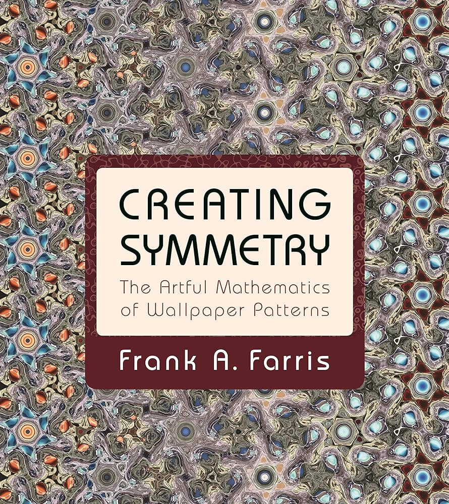{fig-align="center" width="340"}this article delves into the intricate and astounding mathematics that underpins these seemingly simple designs. Through the lens of R programming, we will embark on a journey to uncover the hidden symmetries and patterns that adorn walls and fabrics around the world.# **The Mathematics Behind Wallpaper Patterns**At its core, the study of wallpaper patterns is rooted in group theory and symmetry. These patterns can be classified into 17 distinct groups, each defined by a combination of translations, rotations, reflections, and glide reflections. The mathematical elegance of these symmetries not only provides a systematic way to create intricate designs but also reveals the underlying structure of the patterns we see in our everyday surroundings.# **Bridging Art and Mathematics**The beauty of wallpaper patterns lies in their ability to transform simple geometric rules into complex and visually stunning artwork. By understanding the mathematical principles behind these patterns, we can appreciate the artistry involved in their creation. This article aims to bridge the gap between art and mathematics, showing how mathematical concepts can lead to the creation of beautiful, symmetrical designs.# **Visualizing Symmetry with R Programming**To bring these concepts to life, we will use R programming to generate and animate wallpaper patterns. R, with its powerful visualization libraries, allows us to create detailed and dynamic representations of these patterns. By coding these designs, we not only gain a deeper understanding of the mathematics involved but also create a toolset for artists and designers to experiment with new patterns.In this blogpost, I have provided the complete R source code used to generate each image and animation. For the initial animations, individual images are defined within for loops and subsequently combined into a GIF as the blog post was constructed (as described here). For the final two animations, the full code is supplied, utilizing the [`gifski` package](https://ropensci.org/blog/2018/07/23/gifski-release/), to generate the GIFs.## **Describing Curves with Complex Numbers Using R**Curves, including circles, can be elegantly described using complex functions $z(t)$. R handles complex numbers with ease, making it straightforward to represent and plot both circles and more intricate curves. By leveraging this capability, we can explore a variety of fascinating shapes.### **Understanding Complex Functions**A complex function $z(t)$ can be written in terms of a real parameter $t$. For instance, a circle can be represented as $z(t) = e^{it}$, where $e$ is the base of the natural logarithm, $i$ is the imaginary unit, and $t$ ranges from $0$ to $2\pi$. This representation leverages Euler's formula, $e^{it} = \cos(t) + i\sin(t)$, to describe the circle in the complex plane.### **Creating and Plotting a Circle in R**R’s ability to handle complex numbers allows us to define and manipulate these functions easily. Here’s how we can create and plot a circle using R. Let's start by creating the index $t$. Here's how we begin this journey:```{r}# Define the index tt <-seq(0, 2*pi, length.out =1000)# Example of a simple circle described as a complex functionz <-exp(1i * t)# Plot the circleplot(Re(z), Im(z), type ="l",col ="blue", main ="Circle in the Complex Plane", xlab ="Re(z)", ylab ="Im(z)")```In this example, we:1. Define $t$ as a sequence of values ranging from $0$ to $2\pi$.2. Use the complex exponential function $e^{it}$ to describe the circle.3. Plot the real part of $z$ $(Re(z))$ against the imaginary part $(Im(z))$ to visualize the circle.### **Extending to More Complex Curves**The same approach can be extended to more complex and intriguing curves. By modifying the function $z(t)$, we can create a wide variety of shapes. For example, a spiral can be represented as $z(t) = t e^{it}$, where the radius increases linearly with $t$.```{r}# Describe a spiral as a complex functionz_spiral <- t *exp(1i * t)# Plot the spiralplot(Re(z_spiral), Im(z_spiral), type ="l", col ="red", main ="Spiral in the Complex Plane", xlab ="Re(z)", ylab ="Im(z)")```### Visualization and AnalysisBy leveraging R’s capabilities, we can not only visualize these complex functions but also analyze their properties. Animations, color coding, and interactive plots can enhance our understanding of the underlying mathematics and provide deeper insights into the behavior of these curves.```{r}# Script to draw a circlet =seq(0, 4, l=1000)z =1i^tplot(z)```This creates a vector `t` including the sequence $0$ to $4$ in $1000$ steps. Now to create our circle. Using complex maths, $z(t)=i^t$ with $t$ between $0$ and $4$ describes a complete circle. In R we use `1i` for the complex number $i=\sqrt−1$. So we define a vector `z=1i^t` and make a plot. Note that we don’t need a loop to calculate and plot the entire function. `t` is a vector of $1000$ values, and so when we use `z=1i^t` R creates a vector `z` with $1000$ corresponding values. When we call `plot` with the complex vector `z` R simply plots the imaginary component on the vertical axis against the real component on the horizontal axis. To see the first few `t` and `z` values we could use:```{r}cbind(t,z) |>head()```This approach not only simplifies the mathematical description of these curves but also enhances our ability to visualize and analyze them. Whether we're dealing with familiar geometric shapes or delving into mysterious, intricate curves, R's handling of complex numbers opens up a world of possibilities for mathematical and artistic exploration. With this code, we create a circle in the complex plane, showcasing how R can seamlessly handle and visualize complex numbers. This forms the foundation for further exploration of more complex and intriguing curves.## **Artistic Augmentations**There are a few enhancements we can make to improve the aesthetics of this plot. First, we can remove the axes and annotations for a cleaner look. Additionally, we should ensure the plot is rendered as a continuous line rather than a series of points, and set the aspect ratio to 1 for an accurate representation of the shape. Finally, we can increase the line width (lwd) to 2 for better visibility.Here's how we can amend our script:```{r}t =seq(0, 4, l=1000)z =1i^tplot(z, axes=FALSE, ann=FALSE, type="l", lwd=2, asp=1)```In this updated script:1. `axes = FALSE` removes the axes from the plot.2. `ann = FALSE` removes any annotations such as titles and labels.3. `type = "l"` ensures the plot is drawn as a continuous line.4. `lwd = 2` increases the line width for better visual appeal.5. `asp = 1` sets the aspect ratio to 1, ensuring the plot is not distorted.These adjustments make the plot cleaner and more aesthetically pleasing, highlighting the geometric elegance of the circle. This approach can be similarly applied to other complex functions to create visually appealing representations of mathematical shapes.# **A Mystery Curve**## **Complex Exponential and Rotations in the Complex Plane**The fundamental mathematical operation in the code involves complex exponentials. Given a complex number $z(t)$ represented as:$$z(t) = re^{i\theta(t)}$$where $r$ is the amplitude (modulus) and $\theta(t)$ is the phase (argument), this expression can be written as:$$z(t) = r\Big(\cos( \theta(t)) + i \sin(\theta(t))\Big)$$In the code, each circle is defined by:$$z_{\text{circle}}(t) = \text{amp} \times i^{\text{freq} \times t+ \text{phase}}$$where $i^{\theta} = e^{i\theta}$ (using Euler's formula)This represents a rotation in the complex plane:$$z_{\text{circle}}(t) = \text{amp} \times \left(\cos(\text{freq} \times t + \text{phase}) + i\sin(\text{freq} \times t + \text{phase})\right)$$The parameters:- **Amplitude (`amp`)**: The radius of the circle.- **Frequency (`freq`)**: The speed and direction of rotation. Positive frequency rotates counterclockwise, while negative frequency rotates clockwise.- **Phase (`phase`)**: The initial angle or offset.## Superposition of Complex FunctionsThe code combines multiple circles (complex exponential) by adding them together:$$z(t) = z_1(t) + z_2(t) + z_3(t)$$where:$$z_1(t) = 1 \times i^{1 \times t + 0}, \quad z_2(t) = 0.5 \times i^{5 \times t + 0}, \quad z_3(t) = 0.6 \times i^{-7 \times t + 1}$$This sum is another complex function representing the superposition of the individual circles.The superposition principle is fundamental in linear systems, where the resultant wave is the sum of individual waves. In this context, the real and imaginary parts of each component sum up to produce a new trajectory in the complex plane## **Rotational Symmetry and Modular Arithmetic**A key insight into the pattern formed by the superposition is its rotational symmetry, governed by the frequencies of the components. Specifically, an image exhibits $N$-fold rotational symmetry if all component frequencies have the same remainder when divided by $N$:$$\text{freq}_1 \equiv \text{freq}_2 \equiv \dots \equiv \text{freq}_k \mod N$$In the code:$$ 1 \mod 4 = 1, \quad 5 \mod 4 = 1, \quad -7 \mod 4 = 1$$Since all frequencies are congruent to $1$ modulo $4$, the resultant image has $4$-fold rotational symmetry. This symmetry arises because, when the frequencies are congruent modulo $N$, the contributions from each component reinforce each other at regular intervals (every $\frac{2\pi}{N}$ radians).## Trajectory and Cumulative SumsThe animation part of the code visualizes the evolving trajectory by plotting the cumulative sum of the components:$$\text{lps}_j = \sum_{k=0}^{j} z_k(t)$$This cumulative sum represents the point-by-point construction of the path traced by the function in the complex plane. For each frame $j$, the cumulative point $\text{lps}_j$ is plotted, showing the instantaneous position of the point on its trajectory. The red lines and points added in the animation highlight this trajectory as it evolves over time.However, in the context of the code, the cumulative sum (`lps`) is not a sum over different functions $z_k(t)$ but rather a sum over specific points along the path defined by the complex function $z(t)$. To be more accurate, the expression for the cumulative sum in the code can be represented as:$$\text{lps}_j = \sum_{k=0}^{j} \text{circle}_k(t)$$where $\text{circle}_k(t)$ represents the contributions of each of the individual components up to the current index $j$. In the code, this is implemented as:$$\text{lps}_j = \text{cumsum}\left(0, \text{circle}(1,1,0)[j], \text{circle}(0.5,5,0)[j], \text{circle}(0.6,-7,1)[j]\right)$$Each $\text{circle}(\text{amp}, \text{freq}, \text{phase})[j]$ is a specific point on the trajectory determined by the parameter $j$, and the cumulative sum up to this point is visualized in the animation.## Visualizing the Mystery FunctionTo introduce more complexity and mystery to our plot, we can add additional circular motions with varying amplitudes, frequencies, and phases to our existing circle. This approach results in more intricate and fascinating patterns. By plotting this function $z(t) = it + 0.5i^{5t+1}$ we can observe the interplay between the linear and circular components, resulting in a unique and captivating shape. This approach demonstrates how simple modifications to complex functions can lead to rich and visually stunning patterns.### Explanation of the Mystery FunctionThe function $z(t) = it + 0.5i^{5t+1}$ consists of two components:1. The term $1i\times t$ represents a linear increase in the imaginary direction, creating a spiral-like effect.2. The term $0.5 \times 1i^{5t+1}$ adds additional circular motion with an amplitude of $0.5$, a frequency determined by $5t$, and a phase shift of $1$.Let's plot the function $z(t) = it + 0.5i^{5t+1}.$ Here's the script to achieve this:```{r,eval=FALSE}amp=0.5freq=5phase=1z = 1i^t + # Our original circle amp*(1i^(freq*t + phase)) # A new cirlceplot(z, axes=FALSE, ann=FALSE, type="l", lwd=2, asp=1)#____________________________________________________________________# ~~~~~~~~~~~~~~ Animation ~~~~~~~~~~~~~~~~~~~~~~~~library(gifski)# Define the parametersamp <- 0.5freq <- 5phase <- 1t <- seq(0, 4, length.out = 1000)# Define the function to generate the complex function with the given parametersmystery_function <- function(t, amp, freq, phase) { 1i^t + amp * 1i^(freq * t + phase)}# Create the animationsave_gif( lapply(seq(1, 1000, by = 10), function(j) { z <- 1i^t + amp * 1i^(freq * t + phase) plot(z, axes = FALSE, ann = FALSE, type = "l", lwd = 2, asp = 1) lines(c(0, (1i^t)[j], z[j]), lwd = 3, col = "red") points(c(0, (1i^t)[j], z[j]), cex = 2, pch = 20) }), delay = 1 / 30, width = 600, height = 600, gif_file = "mystery_function_animation.gif")```::: {layout-ncol="2"}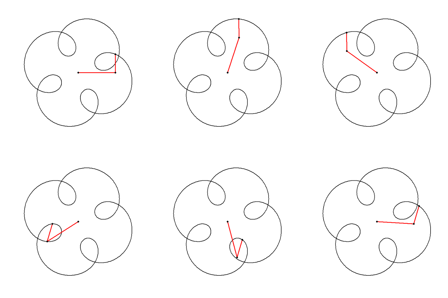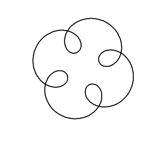{width="534"}:::In this script:1. We define $t$ as a sequence of values from $0$ to $2\pi$.2. We create the mystery function $z(t) = it + 0.5i^{5t+1}$, which introduces additional circular motions with different parameters.3. We plot the function using the same artistic augmentations as before, ensuring the plot is clean and visually appealing.This combination results in a more complex and intriguing pattern, showcasing the power of using complex numbers to create intricate mathematical art.## **Combining Multiple Circles**The following plots, generated by combining three components with frequencies $1$, $5$, and $9$, exhibits $4$-fold rotational symmetry. This symmetry arises due to a specific mathematical property related to the frequencies of the components. According to [Frank A. Farris's](https://en.wikipedia.org/wiki/Frank_Farris) explanation, an image will exhibit $N$-fold rotational symmetry if the frequencies of each component circle yield the same remainder when divided by $N$. Mathematically, this is expressed as all frequencies being congruent modulo $N$. In this case, the frequencies $1$, $5$, and $9$ are all congruent to $1$ modulo $4$:$$1 \;\text{mod}\; 4 =1$$$$5 \; \text{mod}\; 4 =1$$$$9 \; \text{mod}\; 4 =1$$Hence, the resulting image demonstrates $4$-fold rotational symmetry because all the component frequencies are equivalent under modulo $4$ arithmetic. Moreover, negative frequencies can be included in this framework as long as they follow the same rule. For instance, $-7 \mod 4 =1$. Thus, incorporating a frequency of $−7$ will maintain the $4$-fold rotational symmetry of the image.### Formal Algorithm1. **Input Parameters**: Define the amplitudes, frequencies, and phases of the component circles.2. **Frequency Congruence**: Ensure that all frequencies are congruent modulo $N$ (here $N=4$).3. **Circle Function**: Define the function for generating circles in the complex plane.4. **Sum of Circles**: Compute the sum of the component circles.5. **Plotting**: Plot the resulting complex function to visualize the symmetrical pattern.### Steps in the Code1. **Define Circle Function**: $circle(amp,freq,phase)=amp×1i^{(freq×t+phase)}$ where $t$ is a sequence from $0$ to $4$, with $1000$ points.2. **Sum of Circles**: $\text{z=circle(1,1,0)+circle(0.5,5,0)+circle(0.6,9,1)}$3. **Plotting**: - Use `plot` function to visualize the real and imaginary parts of $z$ with appropriate settings for axes, annotations, line type, line width, and aspect ratio.By following this algorithm, the plot generated exhibits the expected $4$-fold rotational symmetry due to the congruence of the component frequencies modulo $4$. To create a more intriguing plot by combining multiple circles, you can define a function to simplify the creation of each circle and then add them together. Here’s how you can approach this in R:```{r,eval=FALSE}circle <- function(amp, freq, phase) amp*1i^(freq*seq(0,4,l=1000)+phase)z = circle(1,1,0) + circle(0.5,5,0) + circle(0.6,9,1)plot(z, axes=FALSE, ann=FALSE, type="l", lwd=2, asp=1)#____________________________________________________________________# ~~~~~~~~~~~~~~ Animation ~~~~~~~~~~~~~~~~~~~~~~~~library(gifski)circle <- function(amp, freq, phase) amp * 1i^(freq * seq(0, 4, length.out = 1000) + phase)save_gif( lapply(seq(1, 1000, by = 2), function(j) { z <- circle(1, 1, 0) + circle(0.5, 5, 0) + circle(0.6, 9, 1) plot(z, axes = FALSE, ann = FALSE, type = "l", lwd = 2, asp = 1) lps <- cumsum(c(0, circle(1, 1, 0)[j], circle(0.5, 5, 0)[j], circle(0.6, 9, 1)[j])) lines(lps, lwd = 3, col = "red") points(lps, cex = 2, pch = 20) }), delay = 1 / 30, width = 600, height = 600, gif_file = "circle_animation.gif")```::: {layout-ncol="2"}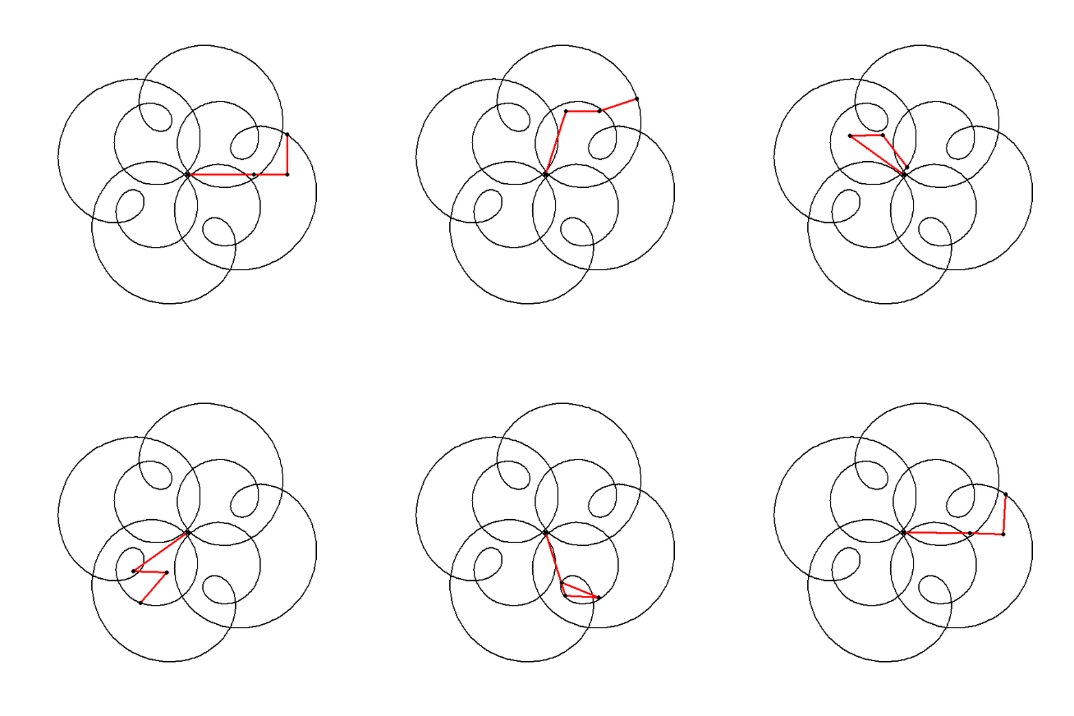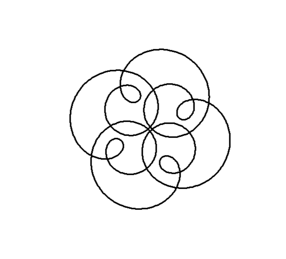{width="524"}:::#### Explanation1. **Function Definition**: `circle` generates a circle in the complex plane given the amplitude (`amp`), frequency (`freq`), and phase (`phase`). - `seq(0, 4, length.out = 1000)` creates a sequence of $1000$ points between $0$ and $4$. - `1i^(freq * seq(0, 4, length.out = 1000) + phase)` generates the complex circle function.2. **Combine Circles**: - `circle(1, 1, 0)` creates the base circle. - `circle(0.5, 5, 0)` adds a circle with different amplitude and frequency. - `circle(0.6, 9, 1)` adds another circle with a different amplitude, frequency, and phase.3. **Plotting**: - `plot(Re(z), Im(z), ...)` plots the real part (`Re(z)`) against the imaginary part (`Im(z)`). - `axes = FALSE` removes the axes. - `ann = FALSE` removes annotations like axis labels and title. - `type = "l"` ensures the plot is drawn as a continuous line. - `lwd = 2` sets the line width for better visibility. - `asp = 1` maintains the aspect ratio, ensuring the plot is not distorted.This code will produce a plot that visualizes the combined effect of three circles in the complex plane, revealing the intricate patterns that emerge from their superposition.```{r,eval=FALSE}library(gifski)circle <- function(amp, freq, phase) amp * 1i^(freq * seq(0, 4, length.out = 1000) + phase)save_gif( lapply(seq(1, 1000, by = 2), function(j) { z <- circle(1, 1, 0) + circle(0.5, 5, 0) + circle(0.6, -7, 1) plot(z, axes = FALSE, ann = FALSE, type = "l", lwd = 2, asp = 1) lps <- cumsum(c(0, circle(1, 1, 0)[j], circle(0.5, 5, 0)[j], circle(0.6, -7, 1)[j])) lines(lps, lwd = 3, col = "red") points(lps, cex = 2, pch = 20) }), delay = 1 / 30, width = 600, height = 600, gif_file = "trajec_animation.gif")```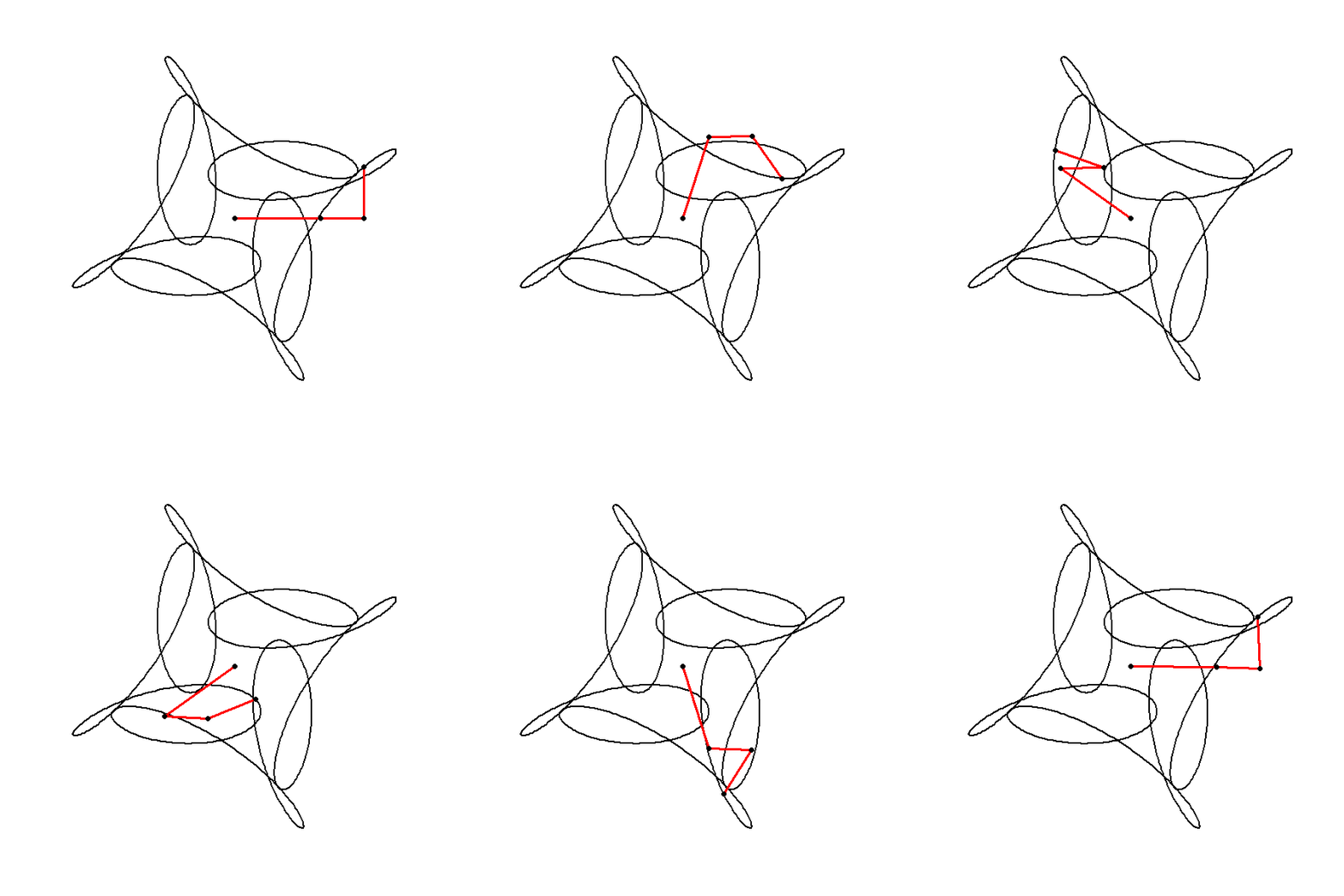{fig-align="center" width="390"}### **Algorithmic Insight**The code provided generates an animated visualization of a complex function composed of three circular components, each defined by its amplitude, frequency, and phase. Here’s a breakdown of the mathematical principles underlying the code:1. **Circle Function**: The `circle` function models each component as a complex exponential function: $$ z(t) = \text{amp} \times i^{\text{freq} \times t+ \text{phase}} $$ - **Amplitude (`amp`)**: Controls the magnitude of the circle. - **Frequency (`freq`)**: Determines the number of oscillations or rotations the circle undergoes over the interval. - **Phase (`phase`)**: Shifts the starting position of the circle along its trajectory.2. **Combination of Circles**: The total complex function `z` is the sum of three such circular components: $$ z(t) = \text{circle}(1, 1, 0) + \text{circle}(0.5, 5, 0) + \text{circle}(0.6, -7, 1) $$ - The first term `circle(1, 1, 0)` is a simple circle with frequency 1. - The second term `circle(0.5, 5, 0)` adds a circle with a higher frequency of 5 and a smaller amplitude of 0.5. - The third term `circle(0.6, -7, 1)` introduces a circle with a negative frequency $(-7)$ and a phase shift of $1$. These components combine to form a more complex path in the complex plane, with the resulting curve reflecting the interplay of the different frequencies, amplitudes, and phase shifts.3. **Symmetry Considerations**: Despite the differences in frequency, the use of congruent modulo arithmetic (as discussed earlier) ensures certain symmetries in the resulting pattern. For instance, the inclusion of a negative frequency still maintains the 4-fold rotational symmetry because $-7 \mod 4 = 1$.### Animation InsightThe animation is constructed to visualize how the complex function evolves over time, showing the dynamic interaction of the three components. Here’s how it works:1. **Frame Generation**: - The code generates $500$ frames (`seq(1, 1000, by = 2)`), with each frame corresponding to a different time point (`j`). - For each frame, the complex function `z` is calculated, and the position of the current point along the path is plotted.2. **Plotting the Path**: - `plot(z, ...)` creates the main plot of the entire trajectory of the function. - `lines(lps, ...)` and `points(lps, ...)` are used to draw and highlight the specific path of the current point (`j`), emphasizing the progression over time. This provides a visual cue of how the components interact dynamically.3. **Cumulative Sum (`cumsum`)**: - The `cumsum` function calculates the cumulative sum of the circle components up to the current time point `j`. This simulates the construction of the trajectory as the animation progresses. - The resulting cumulative points are plotted with red lines and dots, creating a visual of the instantaneous position of the point on its path.4. **GIF Creation**: - `save_gif` combines these frames into a single GIF file, `trajec_animation.gif`, with each frame displayed for $1/30^{\text{th}}$ of a second. - The result is a smooth animation that traces the trajectory of the combined complex function, allowing viewers to see how the path evolves as the components interact.The code effectively demonstrates the rich interplay of multiple circular components in the complex plane, resulting in a visually intricate pattern that evolves over time. The mathematical principles of complex exponential and modular arithmetic are key to understanding the symmetry and structure of the resulting animation. The use of animation enhances the understanding by providing a dynamic visualization of the continuous transformation of the function. We can alter the shape of a curve over time by changing its parameters as we animate. In the code below, an animation is built with the parameter $j$ which varies from 0 to 4 in 100 steps . The phase shift (starting angle) of the third component is set equal to j. In addition, the limits of the plot are now fixed at $(−2,2)$ in both dimensions.```{r,eval=FALSE}library(gifski)circle <- function(amp, freq, phase) amp * 1i^(freq * seq(0, 4, length.out = 1000) + phase)limits <- c(-1, 1) * 2save_gif( lapply(seq(0, 4, length.out = 100)[-1], function(j) { z <- circle(1, 1, 0) + circle(0.5, 5, 0) + circle(0.6, -7, j) plot(z, xlim = limits, ylim = limits, axes = FALSE, ann = FALSE, type = "l", lwd = 2, asp = 1, mar = c(0, 0, 0, 0)) }), delay = 1 / 30, width = 600, height = 600, gif_file = "animation-circ.gif")```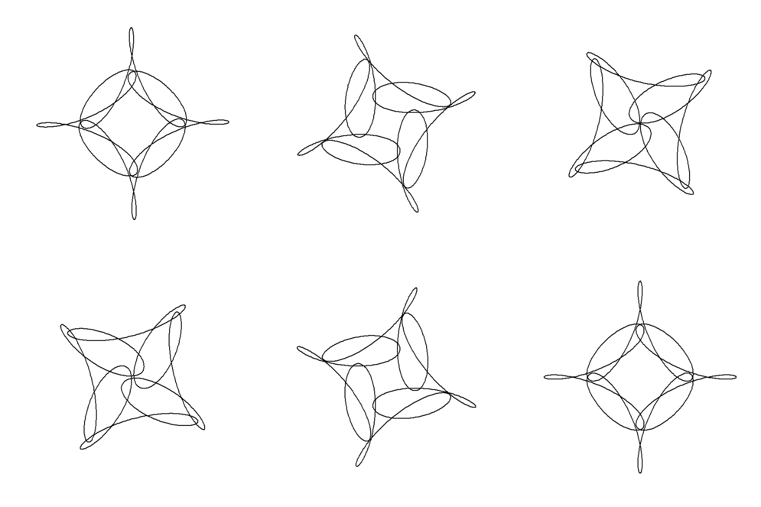{fig-align="center" width="359"}# Mathematical and Artistic Interplay in Plotting Out-of-Order Points## **Mystery Rose**In exploring the artistic potential of mathematical functions, one can introduce a unique form of embellishment by plotting points out of their natural sequence and connecting them with lines. This method adds an element of visual complexity and interest to the underlying mathematical structure.Consider the parameter $t$, which typically varies from $0$ to $4$ in $1000$ steps. This smooth progression generates a continuous curve as each point is plotted sequentially. However, by extending $t$ from $0$ to $40$ in $800$ steps, the points will no longer be plotted in their natural order. Instead, they will appear to skip around the curve in equally spaced intervals, creating a more intricate and seemingly chaotic pattern.Mathematically, this process is analogous to the construction of a Maurer rose, where points are plotted out of order on a rose curve, but here, we apply the technique to a more complex, "mystery" curve. The Maurer rose, named after Peter Maurer, is a geometric figure formed by connecting points that lie on a rose curve with a specific angular step. By altering the sequence of plotted points, the curve becomes a lattice of intersecting lines, revealing hidden symmetries and patterns within the structure.1. **Artistic Fact**: This approach transforms a simple curve into a visually engaging piece of art. The out-of-sequence plotting introduces a rhythm and tension into the image, as the eye is drawn to the unexpected connections between points. The result is an intricate pattern that retains the mathematical elegance of the original curve while introducing an element of surprise and complexity.2. **Mathematical Fact**: From a mathematical perspective, this technique showcases the power of parametric equations and the underlying symmetry of complex functions. By manipulating the sequence in which points are plotted, one can reveal hidden structures and relationships within the function that are not immediately apparent in a traditional, sequential plot.In essence, this technique merges mathematical precision with artistic creativity, demonstrating how altering a simple parameter can lead to a vastly different and visually compelling outcome.```{r,eval=FALSE}library(gifski)circle <- function(amp, freq, phase) amp * 1i^(freq * seq(0, 400, length.out = 799) + phase)limits <- c(-1, 1) * 3save_gif( lapply(seq(0, 4, length.out = 100)[-1], function(j) { z <- circle(1, 1, 0) + circle(1, 6, 0) + circle(1, -9, j) par(bg = "black", mar = c(0, 0, 0, 0)) # Set a black background plot( xlim = limits, ylim = limits, col = "cyan", pch = 20, z, axes = FALSE, ann = FALSE, asp = 1 ) lines(z, col = hsv(0.7, 0.5, 1, 0.5)) # Connect points with lines }), delay = 1 / 30, width = 800, height = 800, gif_file = "circle_animation.gif")```![]()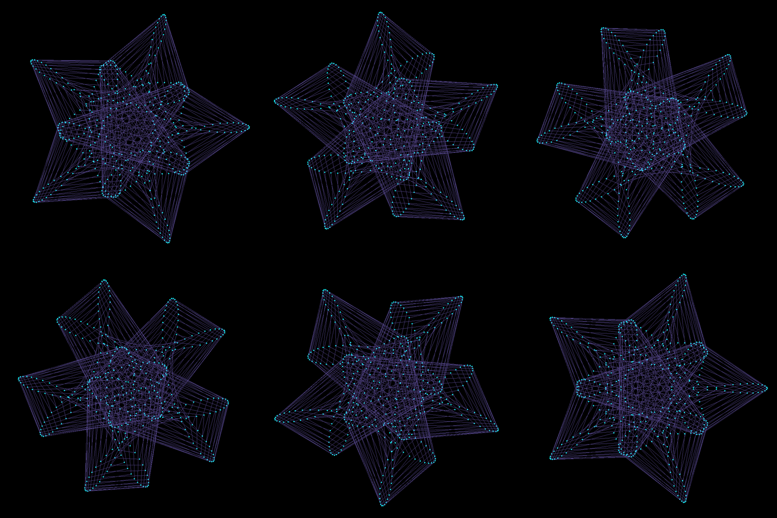{fig-align="center" width="448"}If we modulate the amplitudes of the components with time, we can change the shape of the curve in a very dynamic way. Note in this example, using the `gifski` package explicitly to produce the animation as a `.gif` :```{r,eval=FALSE}library(gifski)circle <- function(amp, freq, phase) amp*1i^(freq*seq(0,400,l=799)+phase)limits=c(-1,1)*2.5# lapply here makes a 'list' of plots, # save_gif turns this list into a gifsave_gif(lapply(seq(0,4,l=500)[-1], function(j){ par(bg="black") z = circle(1,1,0) + circle(sin(pi*j/2),6,0) + circle(cos(pi*j/2),-9,j) hue = (j/4+seq(0,0.5,l=799))%%1 plot(xlim=limits, ylim=limits,col=hsv(hue,.8,1),pch=19, z, axes=FALSE, ann=FALSE, asp=1, mar=c(0,0,0,0)) lines(z,col=hsv(hue[1],.5,1,0.4)) }), delay=1/30,width = 800,height=800, gif_file = "mystery.gif")```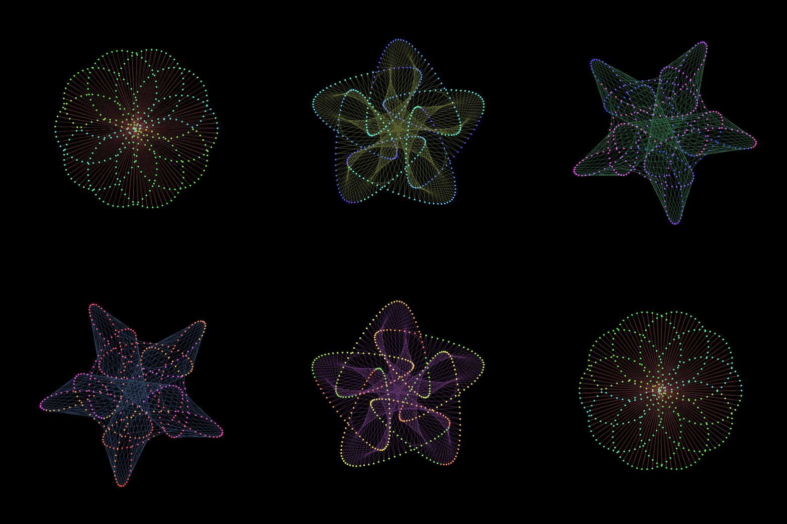{fig-align="center" width="448"}Note the use of `col=` to set the colours of the points and lines. We used `col=hsv(...)` to choose the hue, saturation and value for each point and line.Finally, we can change the frequencies, amplitudes and phases in sync to arrive at this animation. The trick here is to use integer frequencies, and to only change the frequency of a component when its corresponding amplitude is zero. This way our animation can smoothly change its order of rotational symmetry throughout.There are a couple of other nuances in the code below, most important that lines produced by `lines` cannot be different colours, and so I use `segments` instead.```{r,eval=FALSE}library(gifski)circle <- function(amp, freq, phase) amp*1i^(freq*seq(0,600,l=260)+phase)limits=3.5*c(-1,1)li <- seq(0,1,l=500)[-1]save_gif(lapply(1:length(li), function(ai){ a = li[ai]*5; l = sin(pi*(2*a-.5))+1 z<-circle(1,1,0) + circle(l, ceiling(a), -8*a) + circle(l/2-1,ceiling(((-a+2.5)%%5)-5), -4*a) par(mar=c(0,0,0,0), bg="#04010F") hue=(a+(Re(z/10)))%%1 plot(z, col=hsv(hue, 0.65,1), pch=20, lwd=1, cex=1.5, type="p", axes=F, xlim=limits, ylim=limits) z2 <- c(z[-1], z[1]) segments(Re(z), Im(z), Re(z2), Im(z2), col=hsv(hue, 0.65,1,.1), pch=20, lwd=1)}), delay = 1/30, width=800, height=800, gif_file = "mystery2.gif")```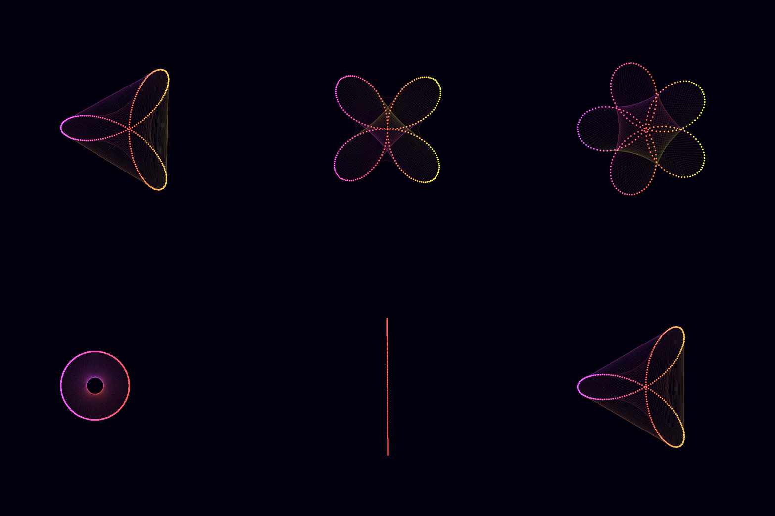{fig-align="center" width="418"}# **Conclusion**The exploration of wallpaper patterns through the lens of mathematics and programming reveals a world where art and science are beautifully intertwined. By leveraging the tools of R programming, we can not only understand but also create and animate these patterns, offering a fresh perspective on the artful mathematics of symmetry. As we delve deeper into the mathematical principles and creative possibilities, we uncover a rich tapestry of designs that adorn our world, reminding us of the inherent beauty and order within mathematical patterns.# **References**- Maurer, Peter M. (August–September 1987). "A Rose is a Rose...". *The American Mathematical Monthly*. **94** (7): 631–645. [CiteSeerX](https://en.wikipedia.org/wiki/CiteSeerX_(identifier) "CiteSeerX (identifier)") [10.1.1.97.8141](https://citeseerx.ist.psu.edu/viewdoc/summary?doi=10.1.1.97.8141). [doi](https://en.wikipedia.org/wiki/Doi_(identifier) "Doi (identifier)"):[10.2307/2322215](https://doi.org/10.2307%2F2322215). [JSTOR](https://en.wikipedia.org/wiki/JSTOR_(identifier) "JSTOR (identifier)") [2322215](https://www.jstor.org/stable/2322215).- [Weisstein, Eric W.](https://en.wikipedia.org/wiki/Eric_W._Weisstein "Eric W. Weisstein") "Maurer roses". MathWorld. (Interactive Demonstrations)- Creating Symmetry [*The Artful Mathematics of Wallpaper Patterns*]{.underline} By Frank A. Farris- ["Mathematical Imagery: Frank Farris: Seeing Symmetry"](http://www.ams.org/publicoutreach/math-imagery/farris). *American Mathematical Society*. Retrieved 2022-04-06.# **Further Readings**- Lamb, Evelyn. ["Impossible Wallpaper and Mystery Curves: Exploring Symmetry in Mathematics and Art"](https://blogs.scientificamerican.com/roots-of-unity/creating-symmetry-frank-farris/). *Scientific American Blog Network*. Retrieved 2022-04-06.- Dobbins, Elizabeth. ["Off the Cuff: Frank A. Farris, professor of mathematics and computer science at Santa Clara University"](https://oberlinreview.org/6083/news/off-the-cuff-frank-a-farris-professor-of-mathematics-and-computer-science-at-santa-clara-university/). *The Oberlin Review*. Retrieved 2020-02-06.{fig-align="center" width="392"}