Dynamics of Julia Sets in Rational Maps
Control and Synchronization with Complex Perturbations
Abstract
This work deals with the study of the dynamical and fractal characteristics of the complex perturbed rational map provided by \(z_{n+1} = \frac{1}{2} \big( z_n + \frac{\lambda}{z_n^q}\big)\). The introduction will first lay out brief historical elaboration of the so-called Julia sets with respect to their significance for studying dynamical systems. It will show how perturbations in rational maps typically afford a cozy ground for complex and varied behavior into more advanced mathematical and computational investigations. The specific method we will implement in this study is the optimal control function method. This method allows for a manipulation of the Julia sets through the controlling of the point at infinity on a rational map. Consequently, the introduction will outline why this methodology will particularly succeed in observing the stability and convergence of dynamical systems and, more generally, mathematical modeling.
The very fact of finding such a nonlinear method makes the realm of coordinated oscillations fresher and more interesting. The driving term associated with the optimal control function has, therefore, been substituted, whereby Julia sets, two belonging to synchronous systems, are evaluated. The buzz that follows this mathematical novelty significantly demands attention given its importance in understanding coupled dynamical systems in different settings. This elaborate introduction, therefore, sets-a-forward framework for the rigorous study of the control mechanisms and synchronization phenomena in complex perturbed rational maps.
Introduction
Fractals are widely studied for their ability to model complex phenomena, and Julia sets are prominent fractal structures in complex dynamics. These sets are defined as the closure of repelling periodic points of rational maps. For a rational map \(R(z) = \frac{P(z)}{Q(z)}\), where \(P\) and \(Q\) are polynomials with \(\text{deg}(P) > \text{deg}(Q)\), infinity acts as a fixed point, and the Julia set is the boundary of the basin of attraction of infinity. The system \(z_{n+1} = \frac{1}{2}\left(z_n + \frac{\lambda}{z_n^q}\right)\), studied here, introduces poles at the origin, transforming the dynamics significantly.
Control of chaotic dynamics, including Julia sets, is critical for many applications. Existing control methods, such as the OGY method and Pyragas feedback, primarily stabilize finite fixed points. In this work, we adopt an optimal control function to regulate Julia sets, treating infinity as a fixed point. Synchronization of Julia sets, essential for understanding relations between different systems, is also explored by aligning their trajectories and fractal structures. This paper contributes to fractal control and synchronization by:
Introducing a control mechanism for Julia sets via the parameter \(k\), with a focus on fractal behavior modification.
Demonstrating synchronization between two Julia sets associated with different parameters in the perturbed rational map.
These advancements provide insights into the interplay between fractal structures and complex dynamics, with implications for chaotic systems and their applications.
In the context of dynamical systems, Julia sets and Mandelbrot sets play a critical role in describing the long-term behavior of iterative processes. Their physical relevance emerges from their ability to model complex systems that exhibit chaotic or fractal-like behavior.
Julia Set and Mandelbrot Sets in Complex Systems
In the context of dynamical systems, Julia sets and Mandelbrot sets play a critical role in describing the long-term behavior of iterative processes. Their physical relevance emerges from their ability to model complex systems that exhibit chaotic or fractal-like behavior.
Julia Sets: The Boundary of Stability
A Julia set \(J(R)\) is a fractal that serves as the boundary between:
Points in the complex plane that exhibit stable, predictable dynamics under a rational map \(R(z)\).
Points that diverge to infinity or exhibit chaotic behavior.
In a physical context:
Julia sets often represent systems that alternate between stable and chaotic regimes.
They serve as models for phase transitions, where the boundary represents critical points between phases.
In fields like optics, Julia sets help describe patterns in nonlinear systems, such as wave front distortions or light propagation through media.
Mandelbrot Sets: A Parameter-Space Map
The Mandelbrot set \(M(c)\), defined as the set of parameters \(c\) for which the orbit of \(z=0\) under the map \(z_{n+1} = z_n^2 + c\) does not escape to infinity, is a tool to explore the global dynamics of complex systems.
It provides a visualization of stability regions in parameter space.
The Mandelbrot set predicts whether perturbations in a system lead to stability or chaos.
Together, Julia and Mandelbrot sets describe critical bifurcations and boundary behaviors, giving insights into systems where small changes in parameters can lead to drastically different outcomes.
Generalized Dynamics
This work describes a generalization of Julia sets and their mathematical framework. This generalization introduces a perturbation parameter \(\lambda\) and a pole at the origin, altering the classical dynamics.
Mathematical Definition:
Perturbed Rational Map:
\[ z_{n+1} = z_n^q + c + \frac{\lambda}{z_n^p} \hspace{1 cm} ...(1) \]
where:
\(q\) controls the degree of the polynomial term.
\(\displaystyle \dfrac{\lambda} {z_n^p}\) introduces a singularity (pole) at the origin.
Impact of \(\lambda\):
For \(\lambda =0\), the map reduces to the classical form \(z_{n+1} = z_n^q + c\), a polynomial.
For \(\lambda \neq 0\), the pole dramatically changes the system’s dynamics, increasing the map’s degree to \(p+q\) and altering the structure of Julia and Mandelbrot sets.
Special Cases:
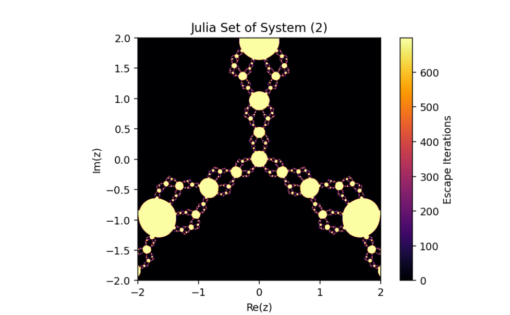
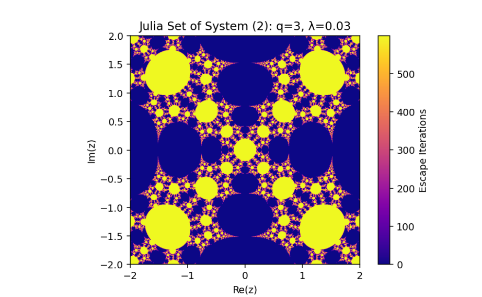
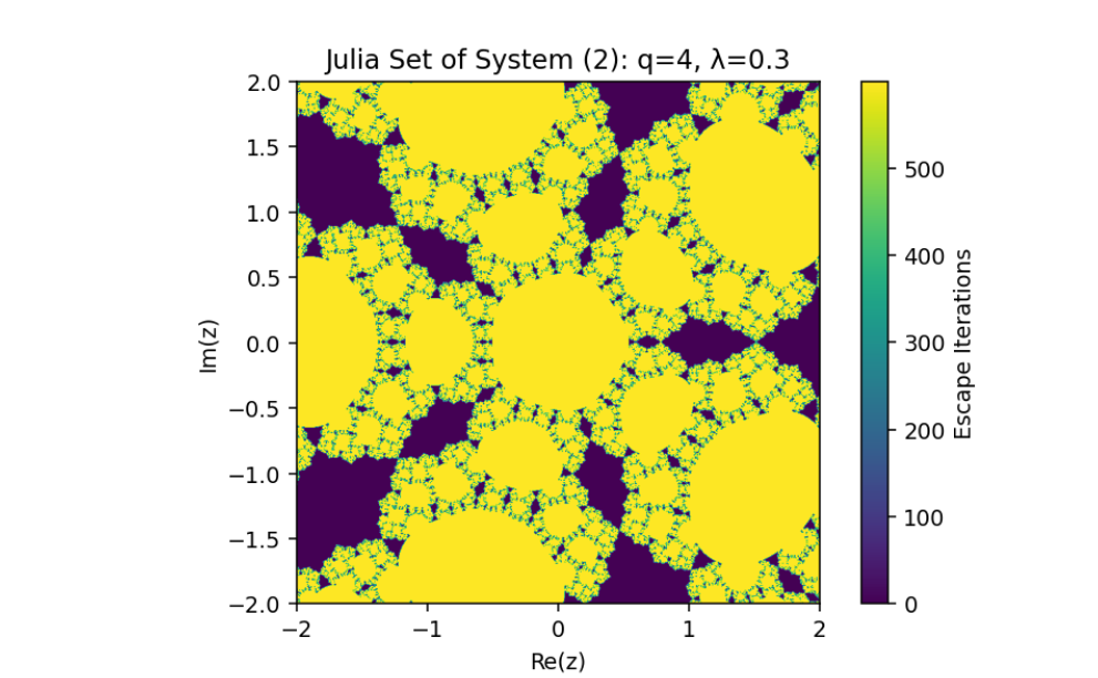
- When \(c = 0\), the study explores how adding a pole affects the Julia set, transforming it from the unit circle (for \(\lambda = 0\) ) to a more complex fractal structure.
Rational Maps and Julia Sets
A rational map \(R(z) = \frac{P(z)}{Q(z)}, \text{where}\; P(z)\; \text {and}\; Q(z)\) are polynomials, forms the basis for studying Julia sets. The degree of \(R(z)\) is defined as \(\max(\deg(P), \deg(Q))\). Julia sets are fractal structures and are defined as:
\[ J(R) = \{z \in \mathbb{C} \mid \text{the family } \{R^n(z)\}_{n \geq 1} \text{ is not normal in the sense of Montel}\}. \]
Equivalently, \(J(R)\) is the closure of the set of repelling periodic points of \(R(z)\). For \(R(z)\), if \(|z| \to \infty\), then \(|R(z)| \to \infty\), making infinity a fixed point. The Julia set \(J(R)\) forms the boundary of the basin of attraction of this fixed point.
Escape Criterion
For a rational map \(R(z)\), an escape criterion determines whether a point belongs to the basin of attraction of infinity. If \(\exists\) \(S > 0\) such that:
\[ |z| > S \implies |R(z)| > |z| \]
then all iterates of \(z\) satisfy \(|R^n(z)| \to \infty\), and \(z\) lies in the basin of attraction of infinity.
Dynamics of the Perturbed Rational Map
The complex perturbed rational map studied is \(z_{n+1} = \frac{1}{2} \left( z_n + \frac{\lambda}{z_n^q} \right),\) where \(q \geq 1\), \(\lambda \in \mathbb{C}\), and \(z \in \mathbb{C}\). Key features include:
\(z_{n+1}\) contains poles at the origin, altering the dynamics of classical Julia sets.
When \(\lambda = 0\), the system reduces to a polynomial map of degree \(q+1\).
This map generalizes rational maps \(R(z) = \frac{P(z)}{Q(z)},\) where \(P(z)\) and \(Q(z)\) are polynomials, by introducing a pole at the origin. This perturbation significantly alters the dynamics and the structure of the Julia sets associated with the map.
Fixed Points and Their Stability
In rational maps, fixed points satisfy \(R(z)=z\). The stability of these fixed points depends on the derivative \(R'(z)\):
Attracting: \(R'(z)<1\),
Repelling: \(R'(z)>1\),
Neutral: \(R'(z)=1\).
In this work, infinity acts as a fixed point, and its behavior is analyzed through escape criteria and control mechanisms.
Control of Julia Set of the Complex Perturbed Rational System
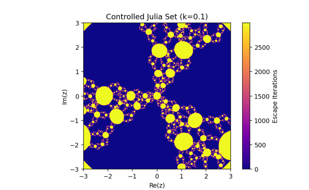
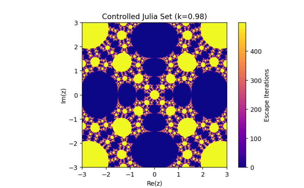
Introducing a control mechanism to Julia sets opens new possibilities for exploring stability, bifurcation, and parameter sensitivity. The controlled rational map introduced earlier is a rich ground for experimentation and understanding dynamical behavior. In this section, we will delve deeper into the computational and algorithmic aspects of controlled Julia sets. A control parameter \(k\) is introduced to modify the dynamics of the map. The controlled map is defined as:
\[ g(z) = f(z) - k \cdot (f(z) - z) \]
Interpretation:
Base Map Contribution: The term \(f(z)\) represents the original rational Julia map.
Feedback Control: The term \(k \cdot (f(z) - z)\) acts as a damping factor. The control parameter \(k\) (with \(0 \leq k \leq 1\)) adjusts the extent to which the new value depends on the previous iteration.
When \(k=0\), \(g(z) = f(z)\), recovering the original Julia map. When \(k=1\), the map becomes stationary.
The Base System and Rational Map:
The base system is:
\[ z_{n+1} = f_{\lambda, q}(z_n) = \frac{1}{2} \left(z_n + \frac{\lambda}{z_n^q}\right) \hspace{1 cm} ...(2) \]
which can also be written as:
\[f_{\lambda, q}(z) = \frac{z^{q+1} + \lambda}{2z^q}.\]
This is a rational map where:
The numerator \(P(z) = z^{q+1} + \lambda\),
The denominator \(Q(z) = 2z^q\).
Since the degree of \(P(z)\) is greater than \(Q(z)\), \(|f_{\lambda, q}(z)| \to \infty\) as \(|z| \to \infty\), and infinity is a fixed point. However, infinity is not an attracting fixed point because the ratio \(\alpha = \frac{|2|}{1}= 2\), which does not satisfy the condition \(|\alpha| < 1\).
Introducing the Nonlinear Control:
To control the dynamics, a nonlinear control term \(u_n\) is introduced:
\[ u_n = -k[f_{\lambda, q}(z_n) - z_n]. \]
The controlled system becomes:
\[ z_{n+1} = f_{\lambda, q}(z_n) + u_n \]
or equivalently:
\[ z_{n+1} = f_{\lambda, q}(z_n) - k[f_{\lambda, q}(z_n) - z_n] \]
Substitute \(f_{\lambda, q}(z_n) = \frac{1}{2} \left(z_n + \frac{\lambda}{z_n^q}\right)\) into the controlled system:
\[ z_{n+1} = \frac{1}{2} \cdot \left(z_n + \frac{\lambda}{z_n^q}\right) - k \cdot \left[\frac{1}{2} \cdot \left(z_n + \frac{\lambda}{z_n^q}\right) - z_n\right] \hspace{1.5 cm} ...(3) \]
\[ \implies z_{n+1} = \frac{1}{2} z_n + \frac{\lambda}{2 z_n^q} - k \left[\frac{1}{2} z_n + \frac{\lambda}{2 z_n^q} - z_n\right] \]
\[ \implies z_{n+1} = \frac{1}{2} z_n + \frac{\lambda}{2 z_n^q} - k \left(-\frac{1}{2} z_n + \frac{\lambda}{2 z_n^q}\right) \]
\[ \implies z_{n+1} = \frac{1}{2} z_n + \frac{k}{2} z_n + \frac{\lambda}{2 z_n^q} - \frac{k \lambda}{2 z_n^q} \]
\[ \implies z_{n+1} = \frac{1+k}{2} z_n + \frac{\lambda (1-k)}{2 z_n^q} \]
\[ \implies z_{n+1} = \frac{(1+k) z_n^{q+1} + \lambda (1-k)}{2 z_n^q} \]
This is a concise symbolic representation called controlled rational map, and we define this following way:
\[\boxed{ R(z)=\frac{(1+k) z_n^{q+1} + \lambda (1-k)}{2 z_n^q}}\]
Fixed Points and Behavior:
Fixed Points: The fixed points are solutions of \(R(z)=z\), which reduce to solving:
\[ \frac{(1+k) z^{q+1} + (1-k)\lambda}{2z^q} = z \]
Rearrange:
\[ (1+k) z^{q+1} + (1-k)\lambda = 2z^{q+1} \]
Factorize:
\[ (1+k - 2)z^{q+1} = -(1-k)\lambda \]
Attracting Fixed Point: If \(∣1+k∣>2\), infinity becomes an attracting fixed point.
Escape Criterion:
That’s how we can write:
\[ |R(z)| > |z| \quad \text{for} \quad |z| > M \]
where \(M\) is a threshold beyond which iterates escape to infinity. Using bounds, the escape criterion simplifies to:
\[ |R(z)| = \left|\frac{(1+k) z^{q+1} + (1-k)\lambda}{2z^q}\right| > |z| \]
The control parameter \(k\) influences the structure of the Julia set.
As \(∣1+k∣>2\), infinity becomes an attracting fixed point, shrinking the Julia set.
The escape criterion ensures iterates either escape to infinity or remain bounded within the Julia set boundary.
Optimal Control Function
The control function modifies the system to regulate its fractal properties. For the perturbed rational map: \(z_{n+1} = R(z_n) + u_n, \; u_{n+1} = -k[R(z_{n+1}) - R(z_n)] + t u_n,\) where \(u_n\) introduces feedback to stabilize desired behaviors.
Key results include:
With \(t=k\), the controlled system simplifies to: \(z_{n+1} = R(z_n) - k[R(z_n) - z_n].\)
This introduces a parameter \(k\) that governs the structure and behavior of the Julia set.
Generalized Map:
Iterative Function:
\[z_{n+1} = z_n^q + c + \frac{\lambda}{z_n^p}\]where:
\(p,q \in \mathbb{Z}^+\), are positive integers.
\(\lambda, c \in \mathbb{C}\) are complex parameters.
\(z_n \in \mathbb{C}\) is the iterated sequence.
Boundedness Criterion:
A point \(z_0\) in the complex plane belongs to the filled Julia set if its orbit \(\{z_0, z_1, z_2, \dots\}\) remains bounded under iteration.
For practical purposes, we compute boundedness using an escape radius \(R\):
If \(|z_n| > R\), the point escapes to infinity.
Otherwise, it is bounded.
Key Parameters:
\(q\): Controls the growth of the polynomial term.
\(\lambda\): Perturbation parameter that introduces singularities at the origin.
\(p\): Governs the strength of the singularity.
\(c\): Determines the central point of the hyperbolic component in the Mandelbrot set.
Mathematical Framework for Visualization
The study relies on the escape-time algorithm to visualize Julia sets:
Initialize a grid of points in the complex plane.
Iterate each point under the map \(z_{n+1} = R(z_n)\).
Assign colors based on the number of iterations required to escape a bounded region.
This technique provides insights into the influence of control parameters \(k\) and synchronization mechanisms on the fractal structure.
Visualization Algorithm: Escape-Time Algorithm
Steps:
Initialize Grid:
- Define a grid of points in the complex plane \(z_0\), e.g., \(x, y \in [-2, 2]\).
Iterative Mapping:
For each \(z_0\), compute its orbit:
\[ z_{n+1} = z_n^q + c + \frac{\lambda}{z_n^p} \]
Escape-Time Calculation:
Track the number of iterations \(n\) required for \(|z_n|\) to exceed a given escape radius \(R\).
Assign a colour to \(z_0\) based on \(n\) (e.g., gradient or palette).
Edge Cases:
Points where \(z_n\) diverges rapidly (\(|z_n| \to \infty\)) are coloured differently.
Points that remain bounded ( \(|z_n| \leq R\) after the maximum iteration) are typically coloured black (belong to the Julia set).
Pseudo-Code for Escape-Time Algorithm
# Input Parameters:
# - grid_size: Number of points in the complex plane grid.
# - max_iter: Maximum number of iterations.
# - R: Escape radius.
# - c, λ: Complex parameters.
# - p, q: Integers controlling the dynamics.

Initialize grid_points = [x + yi for x, y in complex plane range]
Initialize fractal_image = empty array of size [grid_size, grid_size]

for each point z_0 in grid_points:
    z = z_0
    for n = 1 to max_iter:
        if |z| > R:
            fractal_image[z_0] = color_based_on(n)
            break
        else:
            z = z^q + c + λ / z^p
    if |z| <= R after max_iter:
        fractal_image[z_0] = black  # Belongs to the Julia set

Display fractal_image

Synchronization of Julia Sets
Synchronization of Julia sets refers to the fascinating interplay between two distinct dynamical systems, where their fractal structures and trajectories align under specific control conditions. This phenomenon arises in the study of coupled systems, particularly in complex dynamics, where multiple Julia sets, associated with different parameters, exhibit coordinated behavior. Synchronization involves aligning the trajectories and fractal properties of two systems:
Driving System:
\[w_{n+1} = \frac{1}{2} \left( w_n + \frac{\mu}{w_n^p} \right) \text{with parameters}\; p, \mu. \hspace{1 cm} ...(4)\]
Response System:
\[z_{n+1} = R(z_n) - k[R(z_n) - R(w_n)]\]
Synchronization is achieved when the trajectory difference: \(|z_{n+1} - w_{n+1}| \to 0, \text{as}\; k \to 1.\)
Coupling Mechanism
The response system incorporates a coupling term to align its dynamics with the driving system:
\[ w_{n+1} = f(w_n, \lambda_1, q_1) \]
\[ z_{n+1} = f(z_n, \lambda_2, q_2) - k \cdot \left(f(z_n, \lambda_2, q_2) - f(w_n, \lambda_1, q_1)\right) \]
where \(k\) is a control parameter. The coupling ensures that the trajectory of \(z_n\) (response) gradually approaches \(w_n\) (driving). Over time, the Julia sets of the two systems synchronize, exhibiting identical or nearly identical fractal structures.
Why Synchronization Works
Synchronization is feasible because:
Both systems originate from the same functional framework.
Differences are limited to parameter variations (\(\lambda\) , \(q\)).
The coupling mechanism effectively bridges the gap created by these parameter differences, aligning the trajectories and fractal properties.
Now, we’re introducing an additional control parameter \(k\), alongside another parameter \(\mu/w_n^p\), into the iteration of the Julia set. This extends the controlled system to incorporate an extra term involving \(w_n\), which seems to further refine or synchronize the dynamics. The control method is applied to a base system similar to System (3), resulting in the following controlled map:
The equation provided is:
\[ z_{n+1} = \frac{1}{2} \left( z_n + \frac{\lambda}{z_n^q} \right) - k \left[ \frac{1}{2} \left( z_n + \frac{\lambda}{z_n^q} \right) - \frac{1}{2} \left( w_n + \frac{\mu}{w_n^p} \right) \right] \hspace{1 cm} ...(5) \]
where:
\(z_n\): Represents the primary iterated complex variable.
\(w_n\): Represents a secondary complex variable interacting with \(z_n\).
\(\lambda\): A complex parameter controlling the rational map dynamics.
\(\mu\): Another complex parameter that modifies the \(w_n\) dependent term.
\(p,q\): Positive integers controlling the degree of the respective rational maps.
\(k\): A feedback control parameter.
a modified version of a Julia set generated by introducing a control mechanism into the dynamics of a rational map. This mechanism alters the behavior of the system, enabling adjustments to its fractal properties based on a coupling or control parameter \(k\). Let’s break down this system and analyze its mathematical structure:
Base Map Contribution:
\[ \frac{1}{2} \left( z_n + \frac{\lambda}{z_n^q} \right) \]
forms the unperturbed Julia set, as seen in System (2).
Secondary Influence:
\[ \frac{1}{2} \left( w_n + \frac{\mu}{w_n^p} \right) \]
introduces a coupling between the \(z_n\) and \(w_n\) dynamics, with the parameter \(\mu\) adjusting this interaction.
Control Mechanism: The term:
\[ - k \left[ \frac{1}{2} \left( z_n + \frac{\lambda}{z_n^q} \right) - \frac{1}{2} \left( w_n + \frac{\mu}{w_n^p} \right) \right] \]
applies feedback that synchronizes the \(z_n\) and \(w_n\) based maps, creating a controlled fractal structure. The control parameter \(k\) determines the extent of this feedback.
Mathematical Interpretation
This system describes a coupled rational map with feedback control, where:
Coupling: The term involving \(w_n\) and \(\mu/w_n^p\) introduces a synchronized perturbation to the primary Julia set, ensuring dynamic interactions between \(z_n\) and \(w_n\).
Feedback: The parameter \(k\) acts as a regulator, controlling the influence of the coupling term and modifying the convergence or divergence of points in the fractal.
Algorithm to Generate Controlled Julia Sets of System (5)
Key Components
Primary System ( \(z_n\) ) :
\[ z_{n+1} = \frac{1}{2} \left( z_n + \frac{\lambda}{z_n^q} \right) \]
This is the baseline iteration for Julia sets.
Secondary System ( \(w_n\) ):
\[ w_{n+1} = \frac{1}{2} \left( w_n + \frac{\mu}{w_n^p} \right) \]
Represents a synchronized auxiliary system.
Feedback Control:
\[ z_{n+1} \text{ updated as: } z_{n+1} - k \left[ z_{n+1} - w_{n+1} \right] \]
Introduces controlled synchronization between \(z_n\) and \(w_n\), regulated by \(k\).
Steps
Initialize the Complex Grid:
Define the range of the complex plane (\(x\) and \(y\) axes).
Create a meshgrid for both \(z_0\) and \(w_0\) (initial states).
Iterative Process:
For each point on the grid, iterate \(z_n\) and \(w_n\) simultaneously.
Use the control parameter \(k\) to adjust \(z_n\) based on its difference with \(w_n\).
Escape Condition:
- Determine escape times based on the modulus ( \(|z_n| > 2\) or \(|w_n| > 2\) ).
Visualization:
- Map the escape times to a color palette (e.g., viridis or inferno).
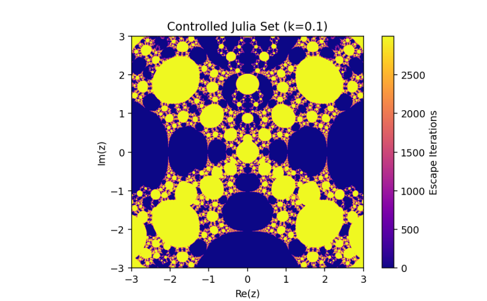
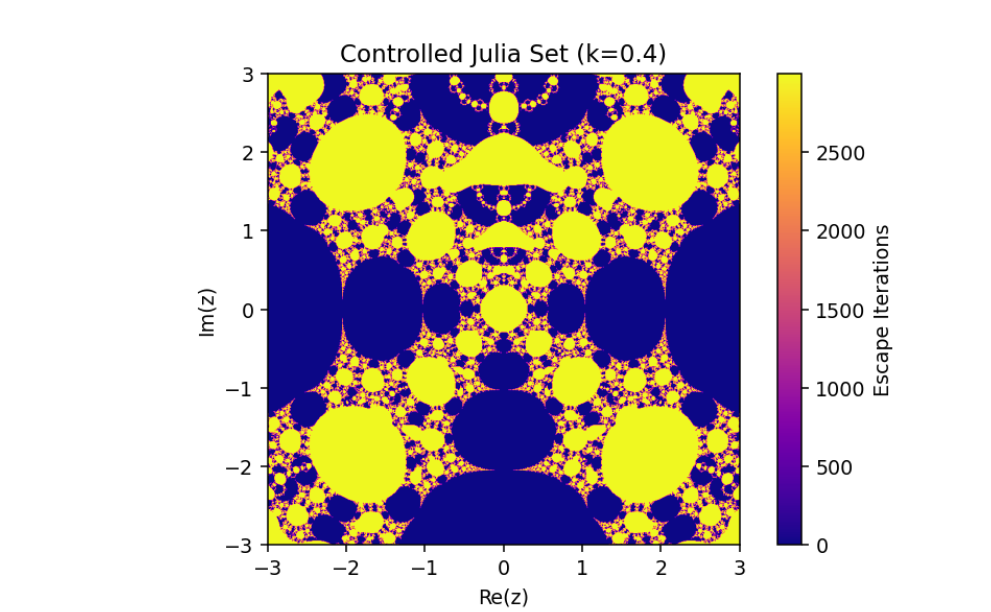
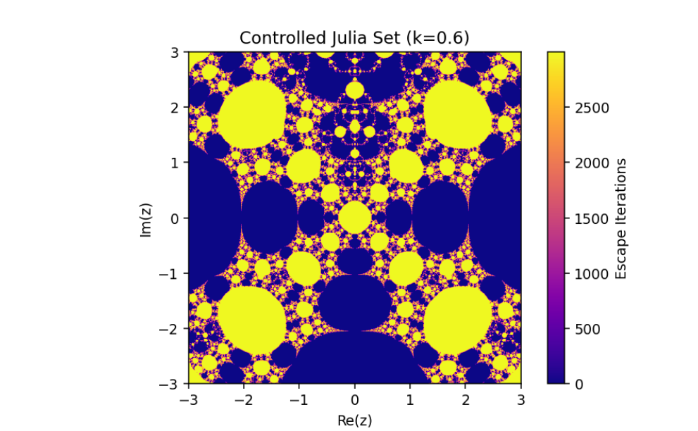
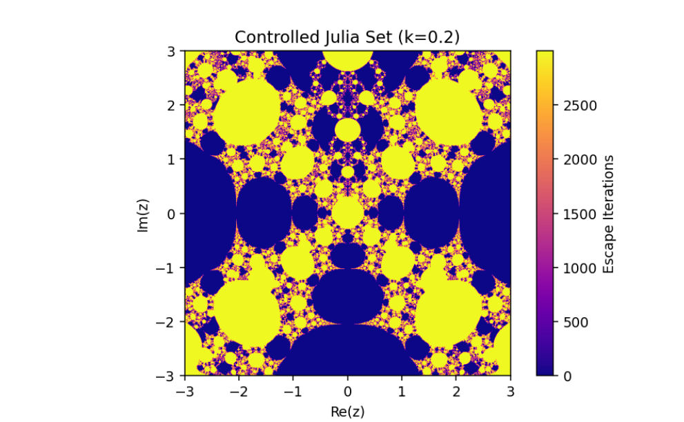
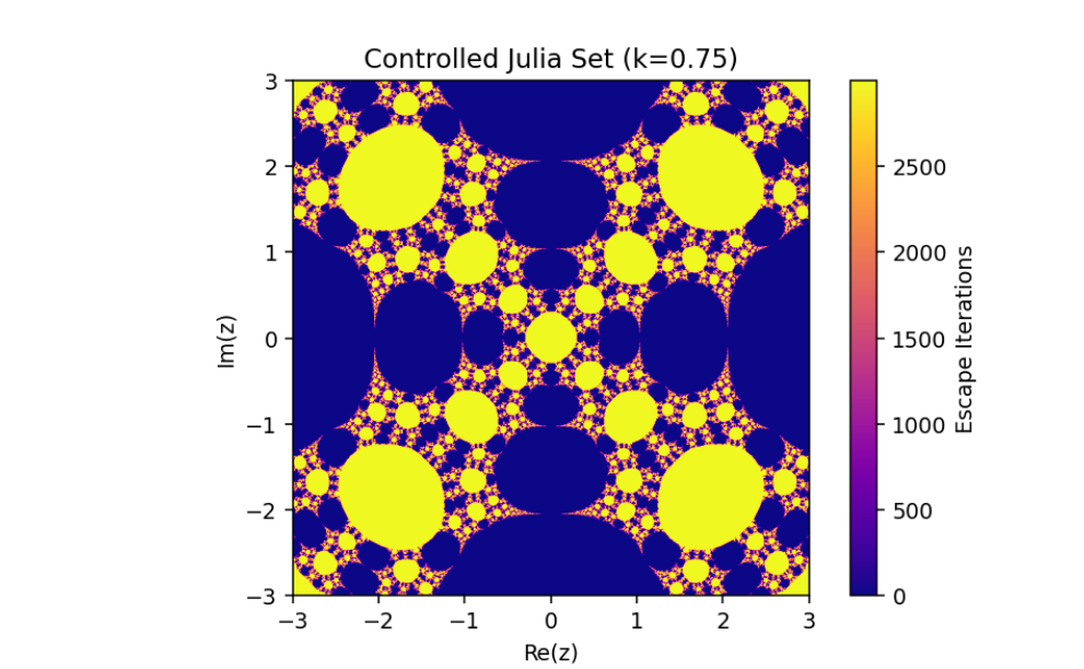
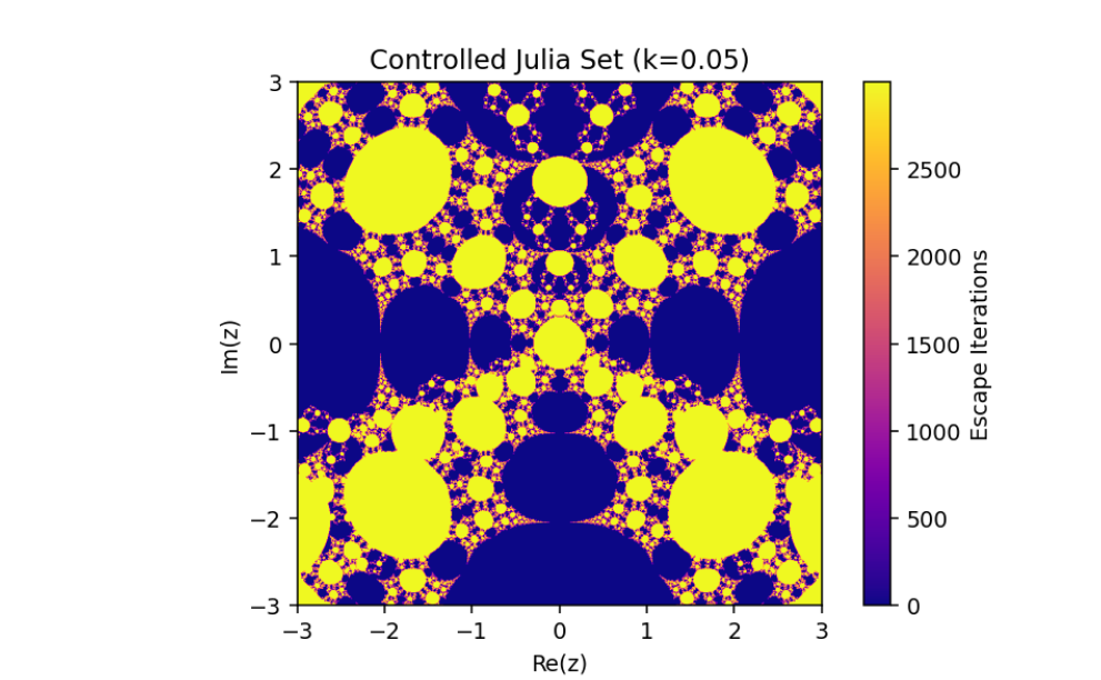
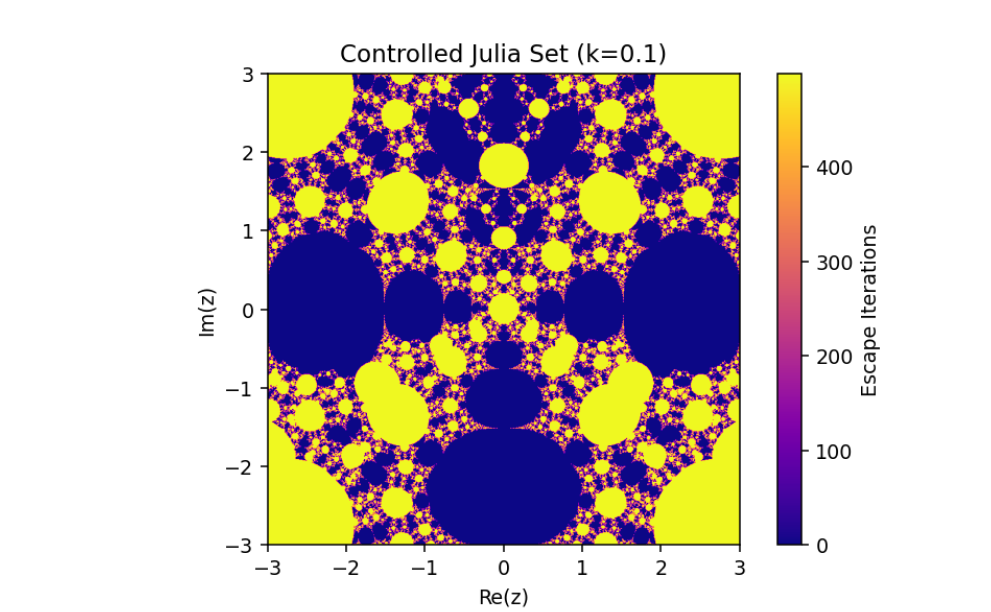
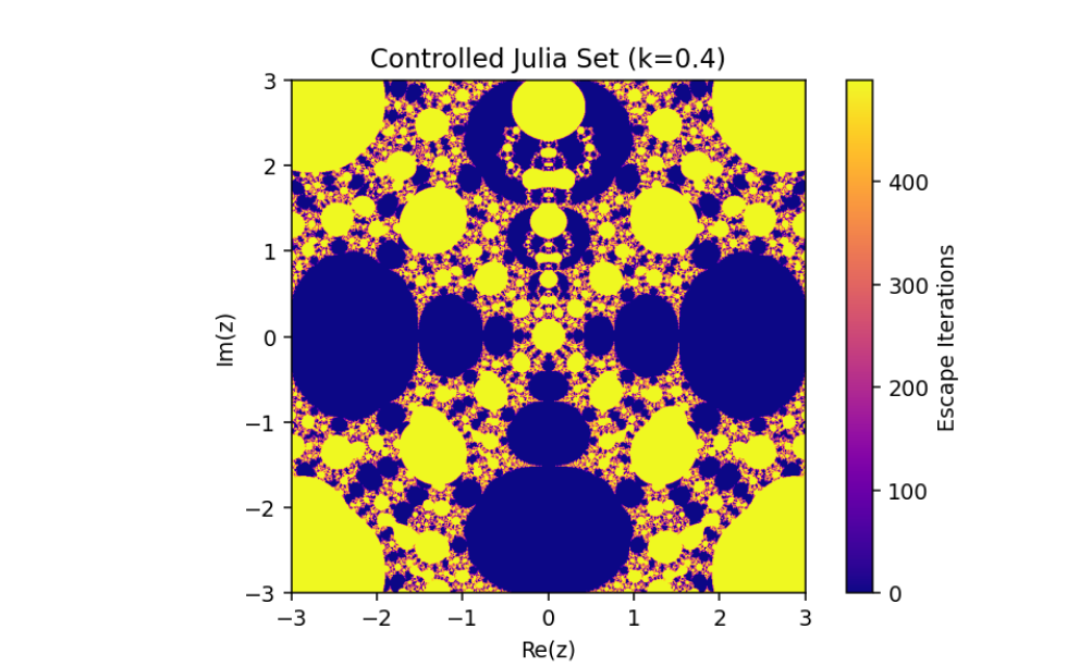
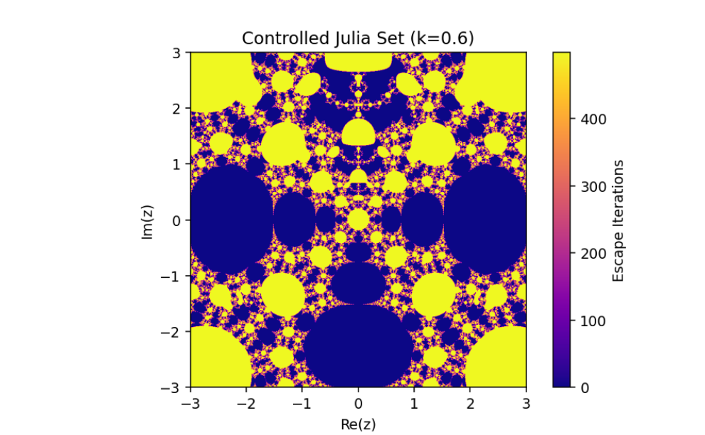
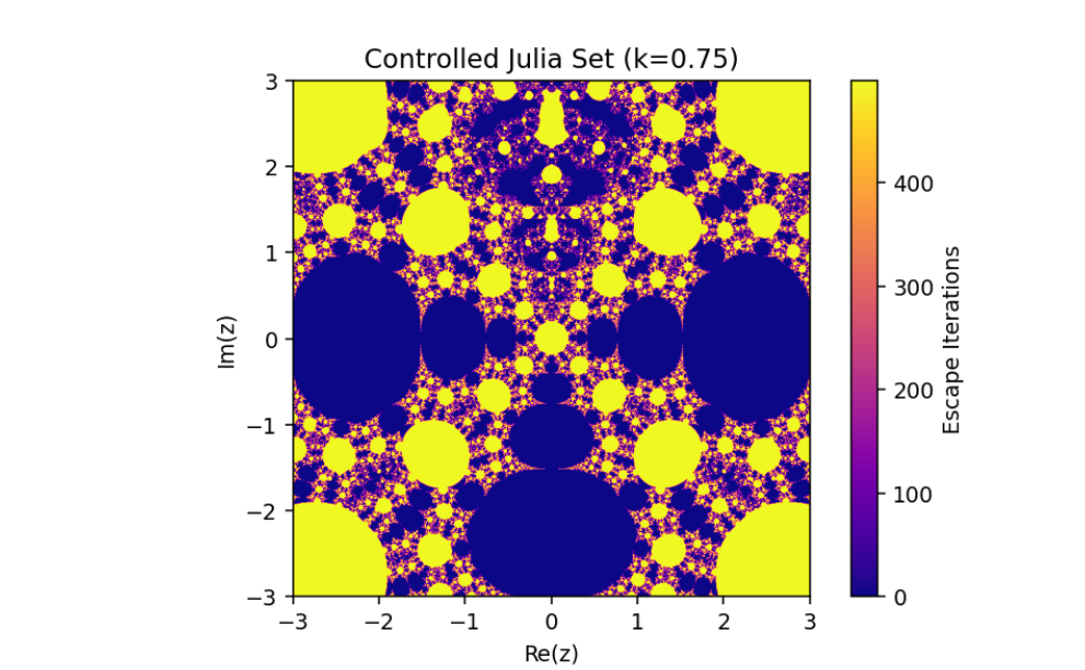
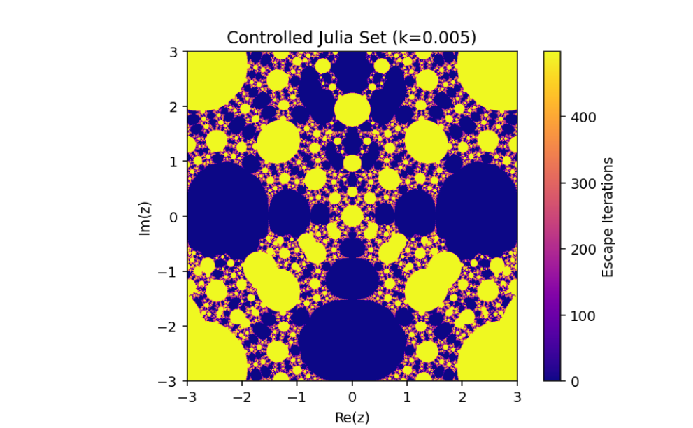
Controlled System (5) when \(q=2,p=2, \lambda =0.073i\)
The changing of Julia sets of the controlled system (5) when \(q=2,p=2, \lambda =0.073i\) demonstrates the dynamic interplay between the driving and response systems under varying control parameter \(k\). As \(k\) evolves, the fractal structures of the Julia sets undergo significant transformations, highlighting the system’s sensitivity to the coupling strength. These variations provide insights into the controlled synchronization of complex dynamical systems, showcasing intricate transitions in the topology of the Julia sets.
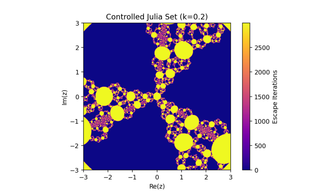
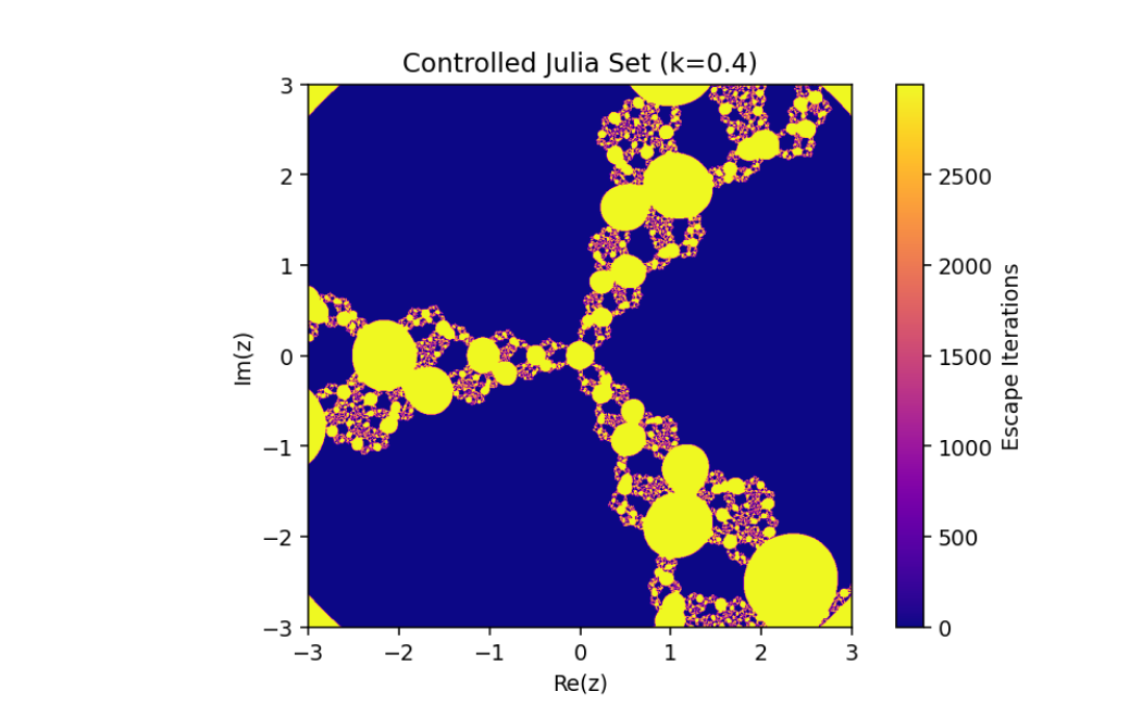
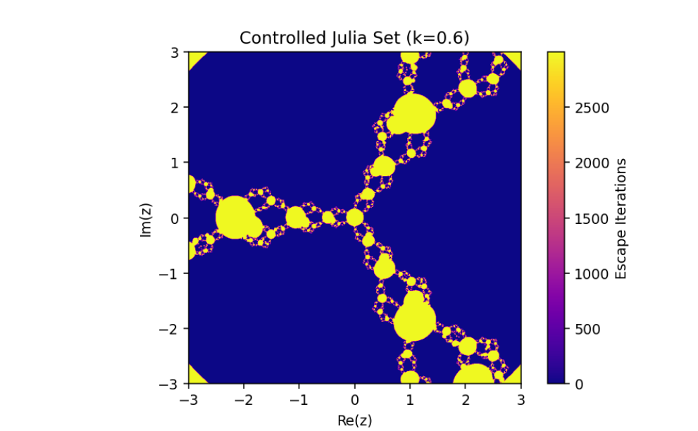
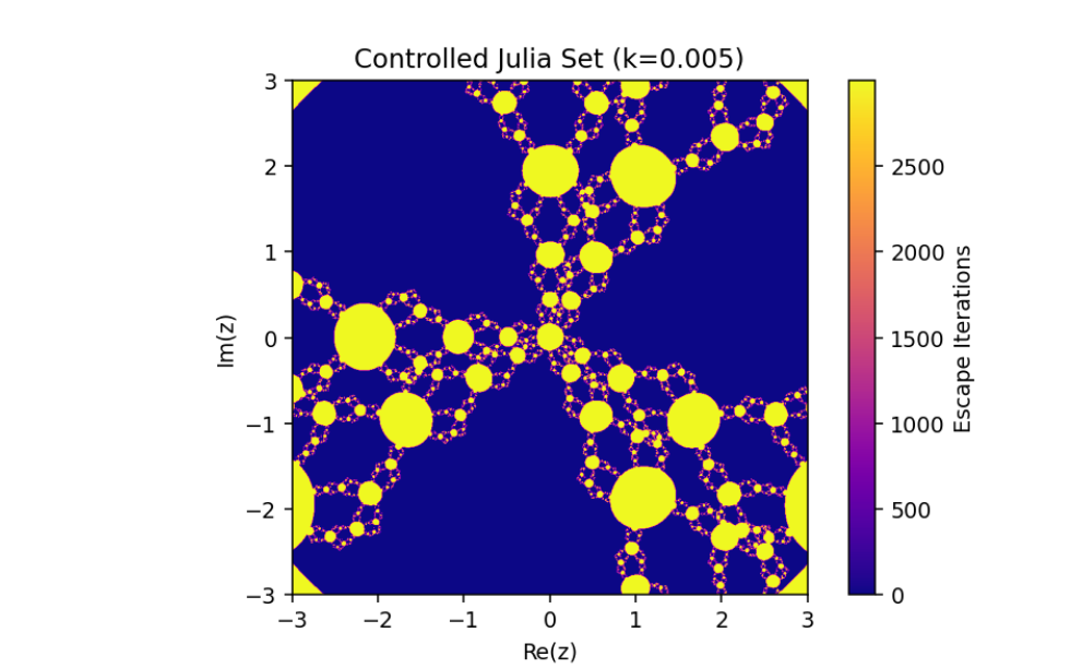

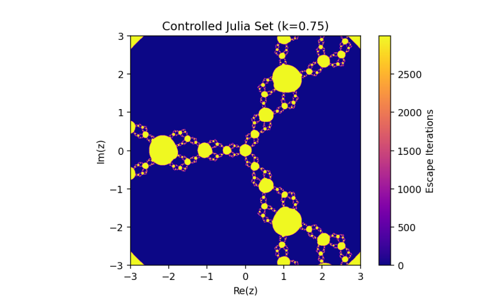

This emphasizes the critical role of feedback control in manipulating complex dynamical systems and offers valuable insights into the sensitive dependence of fractal geometries on system parameters.
Controlled System (5) when \(q=2,p=3, \lambda =0.073i,\mu =0.1\)
The changing of julia sets of the controlled system (5) \(q=2,p=3, \lambda =0.073i,\mu=0.1\) when showcases the dynamic influence of parameter \(k\) on the evolution of the fractal geometry.
This variation emphasizes the sensitivity of the controlled system to specific parameter configurations, resulting in rich, intricate transformations of the Julia sets. These visualizations reveal the complex yet orderly nature of controlled dynamical systems, where stability and chaos coexist in fascinating patterns.
Controlled System (5) when \(q=2,p=3, \lambda =0.073i,\mu=0.03\)
The exploration of the control system \(q=2,p=3, \lambda =0.073i,\mu=0.03\) reveals intricate fractal dynamics driven by the interplay of these parameters. Here, the coupling constants \(\lambda\) and \(\mu\) work together to modulate the system’s feedback and synchronization mechanisms. The influence of \(\mu = 0.03\) introduces additional layers of complexity, shaping the Julia sets into unique geometrical patterns as the control parameter \(k\) is varied.


This combination of parameters highlights the nuanced transitions between stability and chaos in the system, offering deeper insights into the fractal structures and their dependence on the controlled feedback. Such visualizations exemplify the delicate balance between system parameters in driving complex, visually striking dynamics.
Conclusion
In this paper, we have discussed the control and synchronization of Julia sets of the complex perturbed rational maps \(z_{n+1} = \frac{1}{2} \big( z_n + \frac{\lambda}{z_n^q}\big)\), where infinity is regarded as a fixed point to be controlled. In many control methods, the fixed point of the system is finite. However, the fixed point of the complex perturbed rational maps is infinity. In order to avoid the unlimitedness of the fixed point, we take the optimal control function method to control the Julia sets of the complex perturbed rational maps since the fixed point could not appear in the control item. Through the control of Julia sets, we have that Julia sets of the perturbed rational maps are shrinking with the increasing control parameter \(k\). By taking an item in the optimal control function to be the driving item, the synchronization of Julia sets with different system parameters in the perturbed rational maps is also studied. This idea provides a method to discuss the relation and changing of two different Julia sets but not a single one and we can make one Julia set change to be another.
Code References
See the Github Repository Fractal & Research
References
Amritkar, R. E. & Gupte, N. [1993] “Synchronization of chaotic orbits: The effect of a finite time step,” Phys. Rev. E 47, 3889–3895.
Carleson, L. C. & Gamelin, T. W. [1993] Complex Dynamics (Springer-Verlag, NY).
Beck, C. [1999] “Physical meaning for Mandelbrot and Julia sets,” Physica D 125, 171–182.
Zhang, Y. & Sun, W. [2011] “Synchronization and coupling of Mandelbrot sets,” Nonlin. Dyn. 64, 59–63.
Zhang, Y., Sun, W. & Liu, C. [2010] “Control and synchronization of second Julia sets,” Chin. Phys. B 19, 050512.
Kocarev, L. & Parlitz, U. [1996] “Synchronizing spatiotemporal chaos in coupled nonlinear oscillators,” Phys. Rev. Lett. 77, 2206–2209.