Matrix Algebra with R

Vector

Defining Vector in R

A vector is a one-dimensional array of n numbers. A vector is substantially a list of variables, and the simplest data structure in R. A vector consists of a collection of numbers, arithmetic expressions, logical values, or character strings for example. However, each vector must have all components of the same mode, which are called numeric, logical, character, complex, and raw.

A vector is a sequence of data elements of the same type.

Summary

• Vector is a basic data structure in R.

• It is a one-dimensional data structure.

• It holds elements of the same type.

• Members in the vector are called components.

• It is not recursive.

• We can easily convert vectors into data frames or matrices.

• In DataFrame, each column is considered a vector.

Problem Solving

Simple Addition And Scalar Multiplication

Consider \(\text{V}_1\) = The first \(10\) integers, and \(\text{V}_2\) = The next \(10\) integers

V1 <- as.vector(seq(1, 10))
V1

 [1]  1  2  3  4  5  6  7  8  9 10

V2 <- as.vector(seq(11, 20))
V2

 [1] 11 12 13 14 15 16 17 18 19 20

We can add a constant to each element in a vector

V <- V1 + 20
V

 [1] 21 22 23 24 25 26 27 28 29 30

or we can add each element of the first vector to the corresponding element of the second vector

V3 <- V1 + V2
V3

 [1] 12 14 16 18 20 22 24 26 28 30

Transpose

Strangely enough, a vector in R is dimensionless, but it has a length. If we want to multiply two vectors, we first need to think of the vector either as a row or as a column. A column vector can be made into a row vector (and vice versa) by the transpose operation. While a vector has no dimensions, the transpose of a vector is two-dimensional! It is a matrix with \(1\) row and \(n\) columns. (Although the dim command will return no dimensions, in terms of multiplication, a vector is a matrix of \(n\) rows and \(1\) column.)

dim(V1)

NULL

length(V1) # Length of a Vector

[1] 10

TV <- t(V1) # transpose of a Vector
TV

     [,1] [,2] [,3] [,4] [,5] [,6] [,7] [,8] [,9] [,10]
[1,]    1    2    3    4    5    6    7    8    9    10

t(TV)

      [,1]
 [1,]    1
 [2,]    2
 [3,]    3
 [4,]    4
 [5,]    5
 [6,]    6
 [7,]    7
 [8,]    8
 [9,]    9
[10,]   10

dim(t(V1)) # To check the dimession of a vector

[1]  1 10

dim(t(t(V1)))

[1] 10  1

Vector Multiplication

Just as we can add a number to every element in a vector, so can we multiply a number (a”scaler”) by every element in a vector.

VS_Mult <- 4 * V1
VS_Mult

 [1]  4  8 12 16 20 24 28 32 36 40

There are three types of multiplication of vectors in R. Simple multiplication (each term in one vector is multiplied by its corresponding term in the other vector), as well as the inner and outer products of two vectors. Simple multiplication requires that each vector be of the same length. Using the \(\text{V}_1\) and \(\text{V}_2\) vectors from before, we can find the \(10\) products of their elements:

V1

 [1]  1  2  3  4  5  6  7  8  9 10

V2

 [1] 11 12 13 14 15 16 17 18 19 20

V1*V2

 [1]  11  24  39  56  75  96 119 144 171 200

Outer Product

Linear Algebra

The outer product of two coordinate vectors is the matrix whose entries are all products of an element in the first vector with an element in the second vector. If the two coordinate vectors have dimensions \(n\) and \(m\), then their outer product is an \(n × m\) matrix.

\[ \mathbf{v}=\left[\begin{array}{c}v_{1} \\v_{2} \\\vdots \\v_{n}\end{array}\right], \mathbf{w}=\left[\begin{array}{c}w_{1} \\w_{2} \\\vdots \\w_{m}\end{array}\right] \]

Their outer product, denoted \({\mathbf{v} \otimes \mathbf{w}}\) is defined as the \(m \times n\) matrix \(\mathbf{A}\) obtained by multiplying each element of \(\mathbf{v}\) by each element of \(\mathbf{w}.\)

\(\therefore\) The outer product of \(\mathbf{v}\) and \(\mathbf{w}\) is given by,

\[ {\mathbf{v} \otimes \mathbf{w}}=\left[\begin{array}{c}v_{1} \\v_{2} \\\vdots \\v_{n}\end{array}\right] \otimes \left[\begin{array}{c}w_{1} \\w_{2} \\\vdots \\w_{m}\end{array}\right]=\left[\begin{array}{cccc}v_{1} w_{1} & v_{1} w_{2} & \cdots & v_{1} w_{m} \\v_{2} w_{1} & v_{2} w_{2} & \cdots & v_{2} w_{m} \\\vdots & \vdots & \ddots & \vdots \\v_{n} w_{1} & v_{n} w_{2} & \cdots & v_{n} w_{m}\end{array}\right] \]

Example

\(\mathbf{x} = \displaystyle \left[\begin{array}{l}x_{1} \\x_{2}\end{array}\right],\; \mathbf{y} = \left[\begin{array}{l}y_{1} \\y_{2}\end{array}\right], \; \mathbf{z} = \left[\begin{array}{l}z_{1} \\z_{2}\end{array}\right]\)

\[ \mathbf{x} \otimes \mathbf{y} \otimes \mathbf{z}=\begin{aligned}\left[\begin{array}{l}x_{1} \\x_{2}\end{array}\right] \otimes\left[\begin{array}{l}y_{1} \\y_{2}\end{array}\right] \otimes\left[\begin{array}{l}z_{1} \\z_{2}\end{array}\right]=\left[\begin{array}{l}x_{1} \\x_{2}\end{array}\right] \otimes\left[\begin{array}{l}y_{1} z_{1} \\y_{1} z_{2} \\y_{2} z_{1} \\y_{2} z_{2}\end{array}\right] =\left[\begin{array}{l}x_{1} y_{1} z_{1} \\x_{1} y_{1} z_{2} \\x_{1} y_{2} z_{1} \\x_{1} y_{2} z_{2} \\x_{2} y_{1} z_{1} \\x_{2} y_{1} z_{2} \\x_{2} y_{2} z_{1} \\x_{2} y_{2} z_{2}\end{array}\right]\end{aligned} \]

R Programming

The “outer product” of a \(n \times 1\) element vector with a \(1 \times m\) element vector will result in a \(n \times m\) element matrix. (The dimension of the resulting product is the outer dimensions of the two vectors in the multiplication). The vector multiply operator is %*%. In the following equation, the subscripts refer to the dimensions of the variable.

\[ (\mathbf{X} \otimes \mathbf{Y})_{ij} = \mathbf{(XY)}_{ij} \]

Let’s execute by writing some code.

X <- seq(1, 10)
Y <- seq(1, 4)

outer.prod <- X %*% t(Y)
outer.prod

      [,1] [,2] [,3] [,4]
 [1,]    1    2    3    4
 [2,]    2    4    6    8
 [3,]    3    6    9   12
 [4,]    4    8   12   16
 [5,]    5   10   15   20
 [6,]    6   12   18   24
 [7,]    7   14   21   28
 [8,]    8   16   24   32
 [9,]    9   18   27   36
[10,]   10   20   30   40

Outer.Product <- X %*% t(X)
Outer.Product

      [,1] [,2] [,3] [,4] [,5] [,6] [,7] [,8] [,9] [,10]
 [1,]    1    2    3    4    5    6    7    8    9    10
 [2,]    2    4    6    8   10   12   14   16   18    20
 [3,]    3    6    9   12   15   18   21   24   27    30
 [4,]    4    8   12   16   20   24   28   32   36    40
 [5,]    5   10   15   20   25   30   35   40   45    50
 [6,]    6   12   18   24   30   36   42   48   54    60
 [7,]    7   14   21   28   35   42   49   56   63    70
 [8,]    8   16   24   32   40   48   56   64   72    80
 [9,]    9   18   27   36   45   54   63   72   81    90
[10,]   10   20   30   40   50   60   70   80   90   100

A friendly advice to you i.e., For more details about outer product you can use wikipedea as your resource. (Click here)

Inner Product

Linear Algebra

The inner product between two vectors is an abstract concept used to derive some of the most useful results in linear algebra, as well as nice solutions to several difficult practical problems. It is unfortunately a pretty unintuitive concept, although in certain cases we can interpret it as a measure of the similarity between two vectors.

Before giving a definition of the inner product, we need to remember a couple of important facts about vector spaces.

When we use the term “vector” we often refer to an array of numbers, and when we say “vector space” we refer to a set of such arrays. However, if you revise the lecture on vector spaces, you will see that we also gave an abstract axiomatic definition: a vector space is a set equipped with two operations, called vector addition and scalar multiplication, that satisfy a number of axioms; the elements of the vector space are called vectors. In that abstract definition, a vector space has an associated field, which in most cases is the set of real numbers \(\mathbb{R}\) or the set of complex numbers \(\mathbb{C}.\) When we develop the concept of the inner product, we will need to specify the field over which the vector space is defined.

More precisely, for a real vector space, an inner product \(\langle . , \; . \rangle\) satisfies the following four properties. Let \(\mathbf{u, v}\), and \(\mathbf{w}\) be vectors and \(\alpha\) be a scalar, then:

\(\langle \mathbf{u}+\mathbf{v}, \mathbf{w} \rangle = \langle \mathbf{u}, \; \mathbf{w} \rangle\ + \langle \mathbf{v}, \; \mathbf{w} \rangle.\)

\(\langle \alpha\mathbf{v}, \; \mathbf{w} \rangle = \alpha\langle \mathbf{v}, \; \mathbf{w} \rangle.\)

\(\langle \mathbf{v}, \; \mathbf{w} \rangle = \langle \mathbf{w}, \; \mathbf{v} \rangle\)

A vector space together with an inner product on it is called an inner product space. This definition also applies to an abstract vector space over any field.

Formal Definition

An inner product space is a vector space \(V\) over the field \(F\) together with an inner product, that is, a map \(\langle . , \; . \rangle: V\times V \to F\) that satisfies the following three properties for all vectors \(x,y,z \in V\) and all scalars \(a,b \in F.\)

The real numbers \(\mathbb{R}\) are a vector space over \(\mathbb{R}\) that becomes an inner product space with arithmetic multiplication as its inner product: \(\langle x , \; y. \rangle: xy \ \forall \ x,y \in \mathbb{R}\)

More generally, the real\(n\)-space \(\mathbb{R}^n\) with the dot product is an inner product space, an example of a Euclidean vector space.

\[ \Biggl\langle \left[\begin{array}{c}x_{1} \\x_{2} \\\vdots \\x_{n}\end{array}\right] , \; \left[\begin{array}{c}y_{1} \\y_{2} \\\vdots \\y_{n}\end{array}\right] \Biggl\rangle \ = x^T y = \sum_{i=1}^n x_i y_i = x_1y_1+ \ldots+x_ny_n \]

where \(x^T\) is the transpose of \(x.\)

R Programming

The “inner product” is perhaps a more useful operation, for it not only multiplies each corresponding element of two vectors, but also sums the resulting product:

\[ \langle x , \; y \rangle = \sum_{i=1}^n x_iy_i \]

X <- seq(1, 10)
Y <- seq(11, 20)
X

 [1]  1  2  3  4  5  6  7  8  9 10

Y

 [1] 11 12 13 14 15 16 17 18 19 20

in.prod <- t(X) %*% Y
in.prod

     [,1]
[1,]  935

Note that the inner product of two vectors is of length =1 but is a matrix with 1 row and 1 column. (This is the dimension of the inner dimensions (1) of the two vectors.)

Simple Statistics Using Vectors

Although there are built in functions in R to do most of our statistics, it is useful to understand how these operations can be done using vector and matrix operations. Here we consider how to find the mean of a vector, remove it from all the numbers, and then find the average squared deviation from the mean (the variance).

Consider the mean of all numbers in a vector. To find this we just need to add up the numbers (the inner product of the vector with a vector of 1’s) and then divide by n (multiply by the scaler 1/n). First we create a vector of 1s by using the repeat operation. We then show three different equations for the mean.V, all of which are equivalent.

V <- V1
V

 [1]  1  2  3  4  5  6  7  8  9 10

one <- rep(1, length(V)) # To generate a replicated sequence from a specified vector
one

 [1] 1 1 1 1 1 1 1 1 1 1

sum.V <- t(one) %*% V
sum.V

     [,1]
[1,]   55

mean.V <- sum.V * (1/length(V))
mean.V

     [,1]
[1,]  5.5

mean.V <- t(one) %*% V * (1/length(V))
mean.V

     [,1]
[1,]  5.5

mean.V <- t(one) %*% V/length(V)
mean.V

     [,1]
[1,]  5.5

The variance is the average squared deviation from the mean. To find the variance, we first find deviation scores by subtracting the mean from each value of the vector. Then, to find the sum of the squared deviations take the inner product of the result with itself. This Sum of Squares becomes a variance if we divide by the degrees of freedom \((n-1)\) to get an unbiased estimate of the population variance). First we find the mean centered vector:

V - mean.V

 [1] -4.5 -3.5 -2.5 -1.5 -0.5  0.5  1.5  2.5  3.5  4.5

Var.V <- t(V - mean.V) %*% (V - mean.V) * (1/(length(V) - 1))
Var.V

         [,1]
[1,] 9.166667

Matrix Algebra

A matrix is a collection of data elements of the same type arranged in a two-dimensional rectangle. Or, A Matrix is a rectangular arrangement that stores all the memory of linear transformation.

• To create a matrix we must indicate the elements, as well as the number of rows (nrow) and columns (ncol)

• To declare a matrix in R use the function matrix() and a name. As a rule of thumb, matrix names are capitalized. However, R takes even lowercase.

Mathematical Representation

• The size of a matrix is the number of rows and columns in the matrix.

• If \(\mathbf{A}\) is an \(m×n\) matrix, some notations for the matrix include.

  \[ \mathbf{A} = (a_{ij}) = \begin{bmatrix} a_{11} & \cdots & a_{1n} \\ \vdots & \ddots & \vdots \\ a_{m1} & \cdots & a_{mn} \end{bmatrix} \]

• Here \(a_{ij}\) represents the element in the \(i^{\ \text{th}}\) row and the \(j^{\ \text{th}}\) column.

• If \(m=n\), then \(A\) is called a square matrix.

Creating a \(3 \times 3\) matrix

A <- matrix(1:9, nrow = 3, ncol = 3)
A

     [,1] [,2] [,3]
[1,]    1    4    7
[2,]    2    5    8
[3,]    3    6    9

By default, any matrix is created column-wise. To change that we set an additional argumnet byrow = TRUE.

Different Types of Matrix

Diagonal Matrix

MAT <- diag(x = c(1:5, 6, 1, 2, 3, 4), nrow = 4)
MAT

     [,1] [,2] [,3] [,4]
[1,]    1    0    0    0
[2,]    0    2    0    0
[3,]    0    0    3    0
[4,]    0    0    0    4

Symmetric Matrix

A symmetric matrix is a square matrix that is equal to its transpose. In other words, a matrix \(A\) is symmetric if and only if \(A^T=A\), where \(A^T\) denotes the transpose of matrix \(A\).

Mathematically, if you have a symmetric matrix \(A\) of size \(n×n\), its elements are given by \(a_{ij}\)​, and it satisfies the condition:

\(a_{ij}​=a_{ji}\)​

\(\forall i, j\) in the range \(1\le i,j≤n\).

In simpler terms, the entries above and below the main diagonal of a symmetric matrix are mirror images of each other.

MATRIX <- matrix(data = c(1, 2, 2, 1), nrow = 2)
MATRIX

     [,1] [,2]
[1,]    1    2
[2,]    2    1

# Define a symmetric matrix
A <- matrix(c(1, 2, 3, 2, 4, 5, 3, 5, 6), nrow = 3, byrow = TRUE)

# Check if the matrix is symmetric
is_symmetric <- all.equal(A, t(A))  # 't' function transposes the matrix

# Print the matrix and the result
print("Matrix A:")

[1] "Matrix A:"

print(A)

     [,1] [,2] [,3]
[1,]    1    2    3
[2,]    2    4    5
[3,]    3    5    6

print(paste("Is A symmetric? ", is_symmetric))

[1] "Is A symmetric?  TRUE"

A <- matrix(1:9, nrow = 3, ncol = 3, byrow = TRUE)
A

     [,1] [,2] [,3]
[1,]    1    2    3
[2,]    4    5    6
[3,]    7    8    9

It is not necessary to specify both the number of rows and columns. We can only indicate one of them. The number of elements must be a multiple of the number of rows or columns.

A <- matrix(1:9, nrow = 3)
A

     [,1] [,2] [,3]
[1,]    1    4    7
[2,]    2    5    8
[3,]    3    6    9

B <- matrix(1:9, ncol = 3)
B

     [,1] [,2] [,3]
[1,]    1    4    7
[2,]    2    5    8
[3,]    3    6    9

This code creates the matrix \(A\) and then checks if it is symmetric by comparing it to its transpose. The result is a boolean value indicating whether the matrix is symmetric or not. In this case, the output should be “TRUE” since the matrix \(A\) is symmetric.

Orthogonal Matrix

An orthogonal matrix is a square matrix whose transpose is equal to its inverse. In mathematical terms, let \(A\) be an \(n×n\) matrix. The matrix \(A\) is orthogonal if:

\[ A^T⋅A=A⋅A^T=I \]

where \(A^T\) is the transpose of \(A\), \(I\) is the identity matrix.

In simpler terms, an orthogonal matrix is one for which the columns (and, equivalently, the rows) form an orthonormal basis of the Euclidean space. This means that the dot product of any two distinct columns is zero, and the dot product of a column with itself is 1.

# Function to check if a matrix is orthogonal
is_orthogonal <- function(matrix) {
  # Check if the matrix is square
  if (ncol(matrix) != nrow(matrix)) {
    stop("Matrix is not square. Orthogonality applies only to square matrices.")
  }
  
  # Check if the product of the matrix and its transpose is approximately equal to the identity matrix
  is_approx_identity <- all.equal(crossprod(matrix), diag(nrow(matrix)))
  
  return(is_approx_identity)
}

# Example usage
A <- matrix(c(1, 0, 0, 0, 1, 0, 0, 0, 1), nrow = 3, byrow = TRUE)  # Identity matrix, which is orthogonal
B <- matrix(c(1, 1, 0, 0, 1, 0, 0, 0, 1), nrow = 3, byrow = TRUE)  # Not orthogonal

# Check if matrices are orthogonal and print the results
cat("Is matrix A orthogonal? ", is_orthogonal(A), "\n")

Is matrix A orthogonal?  TRUE 

cat("Is matrix B orthogonal? ", is_orthogonal(B), "\n")

Is matrix B orthogonal?  Mean relative difference: 0.75 

This code defines a function is_orthogonal that checks if a given matrix is orthogonal. It then applies this function to two example matrices (A and B) and prints whether each matrix is orthogonal or not. Note that due to numerical precision, the comparison is done using the all.equal function. The crossprod function is used to calculate the crossproduct of a matrix, which is equivalent to \(A^T⋅A\) for the given matrix \(A\)

1. Function Definition (is_orthogonal):

   • This part defines a function named is_orthogonal that takes a matrix as input and checks if it is orthogonal.

   • It first checks if the matrix is square (i.e., the number of columns is equal to the number of rows). If not, it stops the execution and prints an error message.

   • Then, it uses the crossprod function to calculate the crossproduct of the matrix, which is equivalent to \(A^T⋅A\).

   • The all.equal function is used to check if this result is approximately equal to the identity matrix (diag(nrow(matrix))).

   • The result (is_approx_identity) is returned.

2. Example Usage:

   • Two matrices, A and B, are defined. A is an identity matrix, which is known to be orthogonal. B is a matrix that is not orthogonal.

3. Checking and Printing Results:

   • The function is applied to each matrix (is_orthogonal(A) and is_orthogonal(B)).

   • The results are printed using cat, indicating whether each matrix is orthogonal or not.

4. Output:

   • The output will be statements indicating whether matrix A is orthogonal (TRUE) and whether matrix B is orthogonal (FALSE).

This code provides a way to check the orthogonality of a given square matrix and demonstrates its usage with two example matrices.

Various Operation of Matrix

rbind() AND cbind()

rbind() and cbind() allow us to bind vectors in order to create a matrix. The vectors must have the same length

For Example, Declare three vectors.

a <- c(1,2,3,4)
b <- c(10,11,12,13)
c <- c(20,30,40,50)

e <- rbind(a, b, c)
e

  [,1] [,2] [,3] [,4]
a    1    2    3    4
b   10   11   12   13
c   20   30   40   50

The order does not matter.

e <- rbind(c, a, b)
e

  [,1] [,2] [,3] [,4]
c   20   30   40   50
a    1    2    3    4
b   10   11   12   13

Vectors can be repeated.

e <- rbind(a, b, c, a)
e

  [,1] [,2] [,3] [,4]
a    1    2    3    4
b   10   11   12   13
c   20   30   40   50
a    1    2    3    4

It is not necessary to create the vectors first. We can enter them directly in the rbind() function.

e <- rbind(c(1,2,3), c(7,8,9), c(2,3,4))
e

     [,1] [,2] [,3]
[1,]    1    2    3
[2,]    7    8    9
[3,]    2    3    4

If we use cbind() the vectors will be columns.

e <- cbind(a, b, c)
e

     a  b  c
[1,] 1 10 20
[2,] 2 11 30
[3,] 3 12 40
[4,] 4 13 50

Naming The Rows and Columns of a Matrix

e <- matrix(c(1,2,3,4,5,6), nrow = 2, 
            dimnames = list(c("row1", "row2"), 
                            c("col1", "col2", "col3")))
e

     col1 col2 col3
row1    1    3    5
row2    2    4    6

Using the functions rownames() and colnames()

M <- matrix(c(6,1,2,3,0,7), nrow = 2)
rownames(M) <- c("row1", "row2")
colnames(M) <- c("col1", "col2", "col3")
M

     col1 col2 col3
row1    6    2    0
row2    1    3    7

A matrix is just a two-dimensional (rectangular) organization of numbers. It is a vector of vectors. For data analysis, the typical data matrix is organized with columns representing different variables and rows containing the responses of a particular subject. Thus, a \(10 \times 4\) data matrix (10 rows, 4 columns) would contain the data of 10 subjects on 4 different variables. Note that the matrix operation has taken the numbers 1 through 40 and organized them column-wise. That is, a matrix is just a way (and a very convenient one at that) of organizing a vector. R provides numeric row and column names (e.g., [1,] is the first row, [,4] is the fourth column, but it is useful to label the rows and columns to make the rows (subjects) and columns(variables) distinction more obvious.

xij <- matrix(seq(1:40), ncol = 4)
rownames(xij) <- paste("S", seq(1, dim(xij)[1]), sep = "")
colnames(xij) <- paste("V", seq(1, dim(xij)[2]), sep = "")
xij

    V1 V2 V3 V4
S1   1 11 21 31
S2   2 12 22 32
S3   3 13 23 33
S4   4 14 24 34
S5   5 15 25 35
S6   6 16 26 36
S7   7 17 27 37
S8   8 18 28 38
S9   9 19 29 39
S10 10 20 30 40

Just as the transpose of a vector makes a column vector into a row vector, so does the transpose of a matrix swap the rows for the columns. Note that now the subjects are columns and the variables are the rows.

t(xij)

   S1 S2 S3 S4 S5 S6 S7 S8 S9 S10
V1  1  2  3  4  5  6  7  8  9  10
V2 11 12 13 14 15 16 17 18 19  20
V3 21 22 23 24 25 26 27 28 29  30
V4 31 32 33 34 35 36 37 38 39  40

Matrix Addition

The previous matrix is rather uninteresting, in that all the columns are simple products of the first column. A more typical matrix might be formed by sampling from the digits \(0-9\). For the purpose of this demonstration, we will set the random number seed to a memorable number so that it will yield the same answer each time.

set.seed(123)
Xij <- matrix(sample(seq(0, 9), 40, replace = TRUE), ncol = 4)
rownames(Xij) <- paste("S", seq(1, dim(Xij)[1]), sep = "")
colnames(Xij) <- paste("V", seq(1, dim(Xij)[2]), sep = "")
print(Xij)

    V1 V2 V3 V4
S1   2  4  8  9
S2   2  2  2  6
S3   9  8  3  4
S4   1  8  0  6
S5   5  8  6  4
S6   4  2  4  5
S7   3  7  9  8
S8   5  9  6  1
S9   8  6  8  4
S10  9  9  8  7

Just as we could with vectors, we can add, subtract, muliply or divide the matrix by a scaler (a number with out a dimension).

Xij + 4

    V1 V2 V3 V4
S1   6  8 12 13
S2   6  6  6 10
S3  13 12  7  8
S4   5 12  4 10
S5   9 12 10  8
S6   8  6  8  9
S7   7 11 13 12
S8   9 13 10  5
S9  12 10 12  8
S10 13 13 12 11

round((Xij + 4)/3, 2)

      V1   V2   V3   V4
S1  2.00 2.67 4.00 4.33
S2  2.00 2.00 2.00 3.33
S3  4.33 4.00 2.33 2.67
S4  1.67 4.00 1.33 3.33
S5  3.00 4.00 3.33 2.67
S6  2.67 2.00 2.67 3.00
S7  2.33 3.67 4.33 4.00
S8  3.00 4.33 3.33 1.67
S9  4.00 3.33 4.00 2.67
S10 4.33 4.33 4.00 3.67

We can also multiply each row (or column, depending upon order) by a vector.

V

 [1]  1  2  3  4  5  6  7  8  9 10

Xij * V

    V1 V2 V3 V4
S1   2  4  8  9
S2   4  4  4 12
S3  27 24  9 12
S4   4 32  0 24
S5  25 40 30 20
S6  24 12 24 30
S7  21 49 63 56
S8  40 72 48  8
S9  72 54 72 36
S10 90 90 80 70

Matrix Multiplication

Matrix multiplication is a combination of multiplication and addition. For a matrix \(X_{m \times n}\) of dimensions \(m\times n\) and \(Y_{n \times p}\) of dimension \(n \times p\), the product, \(XY_{m \times p}\) is a \(m \times p\) matrix where each element is the sum of the products of the rows of the first and the columns of the second. That is, the matrix \(XY_{m \times p}\) has elements \(xy_{ij}\) where each

\[ xy_{ij}= \sum_{k=1}^{n} x_{ik} \ y_{jk} \]

Consider our matrix Xij with 10 rows of 4 columns. Call an individual element in this matrix \(x_{ij}.\)We can find the sums for each column of the matrix by multiplying the matrix by our “one” vector with Xij. That is, we can find \(\displaystyle \sum _{i=1}^N X_{ij}\) for the j columns, and then divide by the number (n) of rows. (Note that we can get the same result by finding colMeans(Xij). We can use the dim function to find out how many cases (the number of rows) or the number of variables (number of columns). dim has two elements: dim(Xij)[1] = number of rows, dim(Xij)[2] is the number of columns.

dim(Xij)

[1] 10  4

n <- dim(Xij)[1]
one <- rep(1, n)
one

 [1] 1 1 1 1 1 1 1 1 1 1

x.means <- (t(one) %*% Xij)/n
x.means

      V1  V2  V3  V4
[1,] 4.8 6.3 5.4 5.4

A built in function to find the means of the columns is colMeans. (See rowMeans for the equivalent for rows.)

colMeans(Xij)

 V1  V2  V3  V4 
4.8 6.3 5.4 5.4 

Variances and covariances are measures of dispersion around the mean. We find these by first subtracting the means from all the observations. This means centered matrix is the original matrix minus a matrix of means. To make them have the same dimensions we premultiply the means vector by a vector of ones and subtract this from the data matrix.

X.diff <- Xij - one %*% x.means
X.diff

      V1   V2   V3   V4
S1  -2.8 -2.3  2.6  3.6
S2  -2.8 -4.3 -3.4  0.6
S3   4.2  1.7 -2.4 -1.4
S4  -3.8  1.7 -5.4  0.6
S5   0.2  1.7  0.6 -1.4
S6  -0.8 -4.3 -1.4 -0.4
S7  -1.8  0.7  3.6  2.6
S8   0.2  2.7  0.6 -4.4
S9   3.2 -0.3  2.6 -1.4
S10  4.2  2.7  2.6  1.6

To find the variance/covariance matrix, we can first find the the inner product of the means centered matrix X.diff = Xij - X.means t(Xij-X.means) with itself and divide by \(n-1\). We can compare this result to the result of the cov function (the normal way to find covariances).

X.cov <- t(X.diff) %*% X.diff/(n - 1)
X.cov

          V1        V2       V3        V4
V1  8.844444  3.622222 2.977778 -2.577778
V2  3.622222  7.344444 1.422222 -2.022222
V3  2.977778  1.422222 9.155556  1.600000
V4 -2.577778 -2.022222 1.600000  5.377778

round(X.cov, 2)

      V1    V2   V3    V4
V1  8.84  3.62 2.98 -2.58
V2  3.62  7.34 1.42 -2.02
V3  2.98  1.42 9.16  1.60
V4 -2.58 -2.02 1.60  5.38

Matrix Transposition and Symmetry

In some cases, matrix multiplication is not possible in one configuration but would be possible if the rows and columns of one of the matrices were reversed. This reversal is known as transposition, and is easily done in R.

A    # 2x3 matrix

     [,1] [,2] [,3]
[1,]    1    0    0
[2,]    0    1    0
[3,]    0    0    1

t(A) # 3x2 matrix

     [,1] [,2] [,3]
[1,]    1    0    0
[2,]    0    1    0
[3,]    0    0    1

The transpose of \(\mathbf{A}\) is written as \(\mathbf{A'}\) or \(\mathbf{A}^{\text{T}}\). You’ll see that \(BA\) will not work, but compare this with \(B{A}^T.\)

B %*% t(A)     

     [,1] [,2] [,3]
[1,]    1    1    0
[2,]    0    1    0
[3,]    0    0    1

Note that the dimensionality of \(B{A}^T\), and the elements within this product, differ from those in \(AB\).

Many matrices are square – the two dimensions are the same. Square matrices can have many desirable properties. In particular, square matrices can be symmetric, meaning that they are identical to their transpose. This can be verified by visually comparing a matrix with its transpose or by subtracting one from the other (if symmetric, what should the result be?).

Z <- matrix(data = c(1,2,2,2,4,3,2,3,-4), nrow = 3) # What are the dimensions of this matrix?
Z

     [,1] [,2] [,3]
[1,]    1    2    2
[2,]    2    4    3
[3,]    2    3   -4

t(Z)

     [,1] [,2] [,3]
[1,]    1    2    2
[2,]    2    4    3
[3,]    2    3   -4

Z - t(Z)

     [,1] [,2] [,3]
[1,]    0    0    0
[2,]    0    0    0
[3,]    0    0    0

However, not all square matrices are symmetrical:

P <- matrix(data = c(1,3,-1,-2,2,3,2,2,3), nrow = 3)
P

     [,1] [,2] [,3]
[1,]    1   -2    2
[2,]    3    2    2
[3,]   -1    3    3

t(P)

     [,1] [,2] [,3]
[1,]    1    3   -1
[2,]   -2    2    3
[3,]    2    2    3

P - t(P)

     [,1] [,2] [,3]
[1,]    0   -5    3
[2,]    5    0   -1
[3,]   -3    1    0

We will see many symmetric square matrices (diagonal matrices, identity matrices, variance-covariance matrices, distance matrices, etc.). The diagonal elements of a matrix are often important, and can be easily extracted:

diag(x = Z)

[1]  1  4 -4

This command can also be used to modify the values on the diagonal of a matrix:

Z

     [,1] [,2] [,3]
[1,]    1    2    2
[2,]    2    4    3
[3,]    2    3   -4

diag(x = Z) <- 10; Z

     [,1] [,2] [,3]
[1,]   10    2    2
[2,]    2   10    3
[3,]    2    3   10

Matrix Inversion

An identity matrix is a symmetric square matrix with 1s on the diagonal and 0s elsewhere.  It can be created using the diag() function.  Since an identity matrix is symmetric, the number of rows and columns are the same and you only need to specify one dimension:

I <- diag(x = 4)
I

     [,1] [,2] [,3] [,4]
[1,]    1    0    0    0
[2,]    0    1    0    0
[3,]    0    0    1    0
[4,]    0    0    0    1

Identity matrices are particularly important with respect to matrix inversion. The inverse of matrix \(A\) is a matrix that, when matrix multiplied by \(A\), yields an identity matrix of the same dimensions. The inverse of \(A\) is written as \(A^{-1}\). The solve() function can determine the inverse of a matrix:

Z

     [,1] [,2] [,3]
[1,]   10    2    2
[2,]    2   10    3
[3,]    2    3   10

solve(Z)

            [,1]        [,2]        [,3]
[1,]  0.10655738 -0.01639344 -0.01639344
[2,] -0.01639344  0.11241218 -0.03044496
[3,] -0.01639344 -0.03044496  0.11241218

Z %*% solve(Z) # Verify that the product is an identity matrix

              [,1]          [,2]          [,3]
[1,]  1.000000e+00  2.081668e-17  0.000000e+00
[2,] -1.387779e-17  1.000000e+00 -5.551115e-17
[3,] -2.775558e-17 -1.110223e-16  1.000000e+00

Use the round() function if necessary to eliminate unnecessary decimal places. Inversions only exist for square matrices, but not all square matrices have an inverse.

Q <- Z %*% solve(Z)
Q

              [,1]          [,2]          [,3]
[1,]  1.000000e+00  2.081668e-17  0.000000e+00
[2,] -1.387779e-17  1.000000e+00 -5.551115e-17
[3,] -2.775558e-17 -1.110223e-16  1.000000e+00

round(Q)

     [,1] [,2] [,3]
[1,]    1    0    0
[2,]    0    1    0
[3,]    0    0    1

Sometimes, a matrix has to be inverted to yield something other than an identity matrix.  We can do this by adding a second argument to the solve() function.  Suppose we have the equation \(A{A}^{-1} = B\) and need to calculate \({A}^{-1}\):

A <- matrix(data = c(1,2,2,2,4,3,2,3,-4), nrow = 3)
A

     [,1] [,2] [,3]
[1,]    1    2    2
[2,]    2    4    3
[3,]    2    3   -4

B <- matrix(data = c(1,2,3,2,3,1,3,2,1), nrow = 3)
B

     [,1] [,2] [,3]
[1,]    1    2    3
[2,]    2    3    2
[3,]    3    1    1

A.inv <- solve(A, B)
A.inv

     [,1] [,2] [,3]
[1,]    3   10   49
[2,]   -1   -5  -27
[3,]    0    1    4

A %*% A.inv # Verify the result! What should this be?

     [,1] [,2] [,3]
[1,]    1    2    3
[2,]    2    3    2
[3,]    3    1    1

A matrix is orthogonal if its inverse and its transpose are identical.  An identity matrix is an example of an orthogonal matrix.

Determinant of a Matrix

The determinant of a matrix \(A\), generally denoted by \(|A|\), is a scalar value that encodes some properties of the matrix. In R you can make use of the det function to calculate it.

A

     [,1] [,2] [,3]
[1,]    1    2    2
[2,]    2    4    3
[3,]    2    3   -4

B

     [,1] [,2] [,3]
[1,]    1    2    3
[2,]    2    3    2
[3,]    3    1    1

det(A)

[1] -1

det(B)

[1] -12

Rank of a Matrix

The rank of a matrix is maximum number of columns (rows) that are linearly independent. In R there is no base function to calculate the rank of a matrix but we can make use of the qr function, which in addition to calculating the QR decomposition, returns the rank of the input matrix. An alternative is to use the rankMatrix function from the Matrix package.

qr(A)$rank # 2

[1] 3

qr(B)$rank # 2

[1] 3

# Equivalent to:
library(Matrix)
rankMatrix(A)[1] # 2

[1] 3

Eigenvalues and Eigenvectors

Both the eigenvalues and eigenvectors of a matrix can be calculated in R with the eigen function. On the one hand, the eigenvalues are stored on the values element of the returned list. The eigenvalues will be shown in decreasing order:

eigen(A)$values 

[1]  6.25239614  0.03027609 -5.28267223

eigen(B)$values 

[1]  6 -2  1

On the other hand, the eigenvectors are stored on the vectors element:

eigen(A)$vectors

           [,1]        [,2]       [,3]
[1,] -0.4431126  0.86961106 -0.2177793
[2,] -0.8333967 -0.48910640 -0.2573420
[3,] -0.3303048  0.06746508  0.9414602

eigen(B)$vectors

           [,1]          [,2]       [,3]
[1,] -0.5563486 -7.071068e-01  0.2672612
[2,] -0.6847368  6.926174e-18 -0.8017837
[3,] -0.4707565  7.071068e-01  0.5345225

Eigen Decomposition

Eigen decomposition, also known as spectral decomposition, is a factorization of a square matrix into a canonical form, whereby the matrix is expressed as the product of its eigenvectors and eigenvalues. Given a square matrix \(A\), the eigen decomposition is represented as:

\[ A = V \Lambda V^{−1} \]

• \(V\) is a matrix whose columns are the eigenvectors of \(A\).

• \(\Lambda\) is a diagonal matrix whose diagonal elements are the corresponding eigenvalues of \(A\).

• \(V^{−1}\) is the inverse of matrix \(V\)

In equation form, if \(v_i\) is the \(i^{\ \text{th}}\) column of \(V\) and \(λ_i\)​ is the \(i^{\ \text{th}}\)diagonal element of \(\Lambda\), the eigen decomposition is expressed as:

\[ A . v_i = \lambda_i . v_i \]

# Define a square matrix
A <- matrix(c(4, 1, 2, 3), nrow = 2, byrow = TRUE)

# Perform eigen decomposition
eigen_result <- eigen(A)

# Extract eigenvectors and eigenvalues
eigenvectors <- eigen_result$vectors
eigenvalues <- diag(eigen_result$values)

# Reconstruct the original matrix using eigen decomposition
reconstructed_matrix <- eigenvectors %*% eigenvalues %*% solve(eigenvectors)

# Print the original matrix, eigenvectors, eigenvalues, and the reconstructed matrix
cat("Original Matrix A:\n", A, "\n\n")

Original Matrix A:
 4 2 1 3 

cat("Eigenvectors V:\n", eigenvectors, "\n\n")

Eigenvectors V:
 0.7071068 0.7071068 -0.4472136 0.8944272 

cat("Eigenvalues Lambda:\n", eigenvalues, "\n\n")

Eigenvalues Lambda:
 5 0 0 2 

cat("Reconstructed Matrix:\n", reconstructed_matrix, "\n")

Reconstructed Matrix:
 4 2 1 3 

This code does the following:

1. Defines a square matrix A.

2. Uses the eigen function to perform eigen decomposition, obtaining eigenvectors and eigenvalues.

3. Reconstructs the original matrix using the obtained eigenvectors and eigenvalues.

4. Prints the original matrix, eigenvectors, eigenvalues, and the reconstructed matrix.

You can replace the matrix A with your own square matrix of interest. The result will show you the eigenvectors, eigenvalues, and the reconstructed matrix using eigen decomposition.

Singular Value Decomposition(SVD)

Singular Value Decomposition (SVD) is a factorization method that represents a matrix as the product of three other matrices. Given an \(m×n\) matrix \(A\), its SVD is typically expressed as:

\[ A = U \Sigma V^T \]

where:

• \(U\) is an \(m×m\) orthogonal matrix (left singular vectors).

• \(\Sigma\) is an \(m×n\) diagonal matrix with non-negative real numbers on the diagonal (singular values).

• \(V^T\) is the transpose of an \(n×n\) orthogonal matrix \(V\) (right singular vectors).

The singular value decomposition provides a way to decompose a matrix into its constituent parts, revealing essential information about its structure. SVD is widely used in various applications, including dimensionality reduction, data compression, and solving linear least squares problems.

# Define a matrix
A <- matrix(c(4, 1, 2, 3), nrow = 2, byrow = TRUE)

# Perform singular value decomposition
svd_result <- svd(A)

# Extract U, Sigma, and V
U <- svd_result$u
Sigma <- diag(svd_result$d)
V <- svd_result$v

# Reconstruct the original matrix using singular value decomposition
reconstructed_matrix <- U %*% Sigma %*% t(V)

# Print the original matrix, U, Sigma, V, and the reconstructed matrix
cat("Original Matrix A:\n", A, "\n\n")

Original Matrix A:
 4 2 1 3 

cat("U:\n", U, "\n\n")

U:
 -0.7677517 -0.6407474 -0.6407474 0.7677517 

cat("Sigma:\n", Sigma, "\n\n")

Sigma:
 5.116673 0 0 1.954395 

cat("V:\n", V, "\n\n")

V:
 -0.8506508 -0.5257311 -0.5257311 0.8506508 

cat("Reconstructed Matrix:\n", reconstructed_matrix, "\n")

Reconstructed Matrix:
 4 2 1 3 

This code performs singular value decomposition on a matrix A, extracts the matrices \(U\), \(\Sigma\), and \(V\), and then reconstructs the original matrix. You can replace the matrix A with your own matrix to see the SVD components for your data.

A <- matrix(data = 1:36, nrow = 6, byrow = TRUE)
A

     [,1] [,2] [,3] [,4] [,5] [,6]
[1,]    1    2    3    4    5    6
[2,]    7    8    9   10   11   12
[3,]   13   14   15   16   17   18
[4,]   19   20   21   22   23   24
[5,]   25   26   27   28   29   30
[6,]   31   32   33   34   35   36

y <- svd(x = A)
y

$d
[1] 1.272064e+02 4.952580e+00 8.605504e-15 3.966874e-15 1.157863e-15
[6] 2.985345e-16

$u
            [,1]        [,2]        [,3]         [,4]       [,5]         [,6]
[1,] -0.06954892 -0.72039744  0.66413087 -0.157822256  0.0891868 -0.047523836
[2,] -0.18479698 -0.51096788 -0.63156759 -0.090533384  0.4418991  0.320020543
[3,] -0.30004504 -0.30153832 -0.34646216 -0.006631248 -0.4698923 -0.691497505
[4,] -0.41529310 -0.09210875  0.04190338  0.247123228 -0.6149437  0.614870789
[5,] -0.53054116  0.11732081  0.16119572  0.676892104  0.4260339 -0.197712056
[6,] -0.64578922  0.32675037  0.11079978 -0.669028444  0.1277162  0.001842064

$v
           [,1]        [,2]       [,3]        [,4]        [,5]       [,6]
[1,] -0.3650545  0.62493577  0.5994575  0.02705792  0.21514480  0.2642381
[2,] -0.3819249  0.38648609 -0.4791520 -0.46790018  0.19629562 -0.4665969
[3,] -0.3987952  0.14803642 -0.1071927  0.67748875 -0.49153635 -0.3270449
[4,] -0.4156655 -0.09041326 -0.2351992 -0.33258158 -0.51273132  0.6246800
[5,] -0.4325358 -0.32886294 -0.2887029  0.36900805  0.63916519  0.2769719
[6,] -0.4494062 -0.56731262  0.5107893 -0.27307296 -0.04633795 -0.3722482

Solving System of Linear Equation in R

A system of linear equations (or linear system) is a collection of one or more linear equations involving the same variables.

Use R Package matlib()

A collection of matrix functions for teaching and learning matrix linear algebra as used in multivariate statistical methods. These functions are mainly for tutorial purposes in learning matrix algebra ideas using R. In some cases, functions are provided for concepts available elsewhere in R, but where the function call or name is not obvious. In other cases, functions are provided to show or demonstrate an algorithm. In addition, a collection of functions are provided for drawing vector diagrams in 2D and 3D.

Q1. Show and plot equations in R. Given equations \(-1x_1 + 1x_2 =-2\) , \(2x_1+2x_2 = 1\)

#install.packages("matlib")
library(matlib)
A <- matrix(c(-1, 2, 1, 2), 2, 2)
b <- c(-2,1)
showEqn(A, b)

-1*x1 + 1*x2  =  -2 
 2*x1 + 2*x2  =   1 

plotEqn(A,b)

Solve(A, b, fractions = TRUE)

x1    =   5/4 
  x2  =  -3/4 

Q2. There is a system of linear equation. Solve \(x,y,z\) and plot these three equation.

\[ 4x -3y +z = -10 \]

\[ 2x+y+3z = 0 \]

\[ -x +2y-5z = 17 \]

A <- matrix(c(4,-3,1,2,1,3,-1,2,-5), nrow = 3, ncol = 3)
B <- c(-10,0,17)
showEqn(A,B)

 4*x1 + 2*x2 - 1*x3  =  -10 
-3*x1 + 1*x2 + 2*x3  =    0 
 1*x1 + 3*x2 - 5*x3  =   17 

Solve(A, B, fractions = TRUE)

x1      =  -13/4 
  x2    =   -3/4 
    x3  =   -9/2 

plotEqn3d(A,B)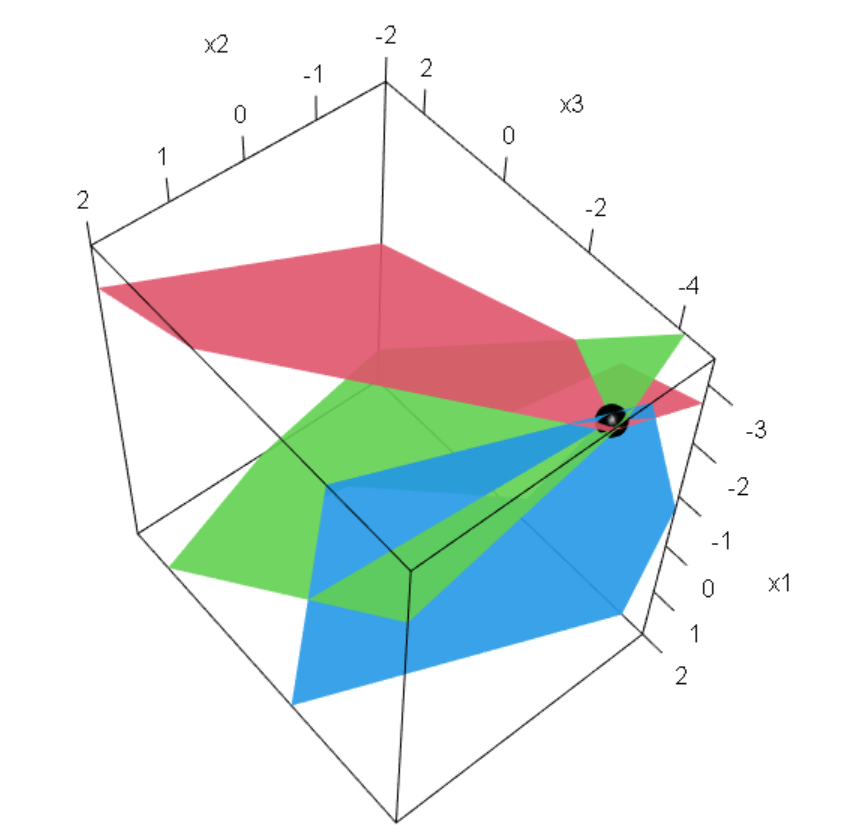

A <- matrix(c(1,2,3, -1, 2, 1), 3, 2)
C <- c(2,1,3)
showEqn(A, C)

1*x1 - 1*x2  =  2 
2*x1 + 2*x2  =  1 
3*x1 + 1*x2  =  3 

plotEqn(A,C)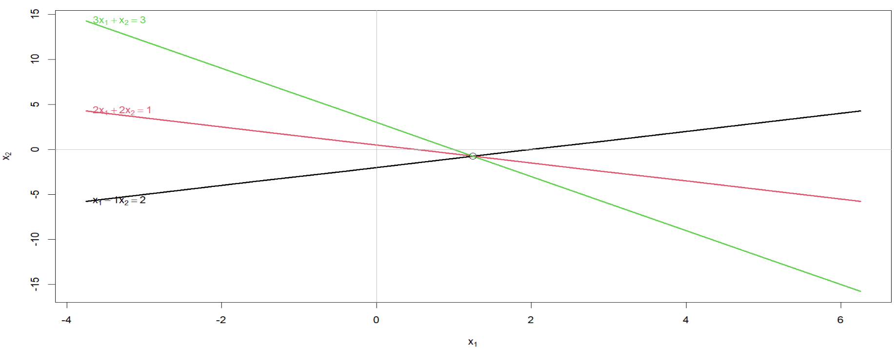

Q3. Solve simultaneous equation using matrix algebra in R. Suppose we have 3 set equations, that we want to solve,

\[ x+2y-4z=40 \]

\[ 2x+3y+5z=50 \]

\[ x+3y+6z=100 \]

A <- matrix(data=c(1,2,-4,2,3,5,1,3,6), nrow=3, ncol = 3)
A

     [,1] [,2] [,3]
[1,]    1    2    1
[2,]    2    3    3
[3,]   -4    5    6

a <- matrix(data=c(40,50,100), nrow=3, ncol = 3)
a

     [,1] [,2] [,3]
[1,]   40   40   40
[2,]   50   50   50
[3,]  100  100  100

showEqn(A,a)

 1*x1 + 2*x2 + 1*x3  =   40 
 2*x1 + 3*x2 + 3*x3  =   50 
-4*x1 + 5*x2 + 6*x3  =  100 

Solve(A,a,fractions = TRUE)

x1      - 70/23*x4  - 70/23*x5  =   -70/23 
  x2   + 560/23*x4 + 560/23*x5  =   560/23 
    x3 - 130/23*x4 - 130/23*x5  =  -130/23 

round(solve(A,a),1)

     [,1] [,2] [,3]
[1,] -3.0 -3.0 -3.0
[2,] 24.3 24.3 24.3
[3,] -5.7 -5.7 -5.7

#transpose of A
t(A)

     [,1] [,2] [,3]
[1,]    1    2   -4
[2,]    2    3    5
[3,]    1    3    6

#inverse of A
round(solve(A),2)

      [,1]  [,2]  [,3]
[1,] -0.13  0.30 -0.13
[2,]  1.04 -0.43  0.04
[3,] -0.96  0.57  0.04

#diagnal matrix of A
diag(A)

[1] 1 3 6

#eigen values of A
eigen(A)

eigen() decomposition
$values
[1]  8.192582  2.807418 -1.000000

$vectors
          [,1]       [,2]       [,3]
[1,] 0.2643057 -0.5595404  0.3333333
[2,] 0.5567734 -0.7151286 -0.6666667
[3,] 0.7874934  0.4189340  0.6666667

plotEqn3d(A,a)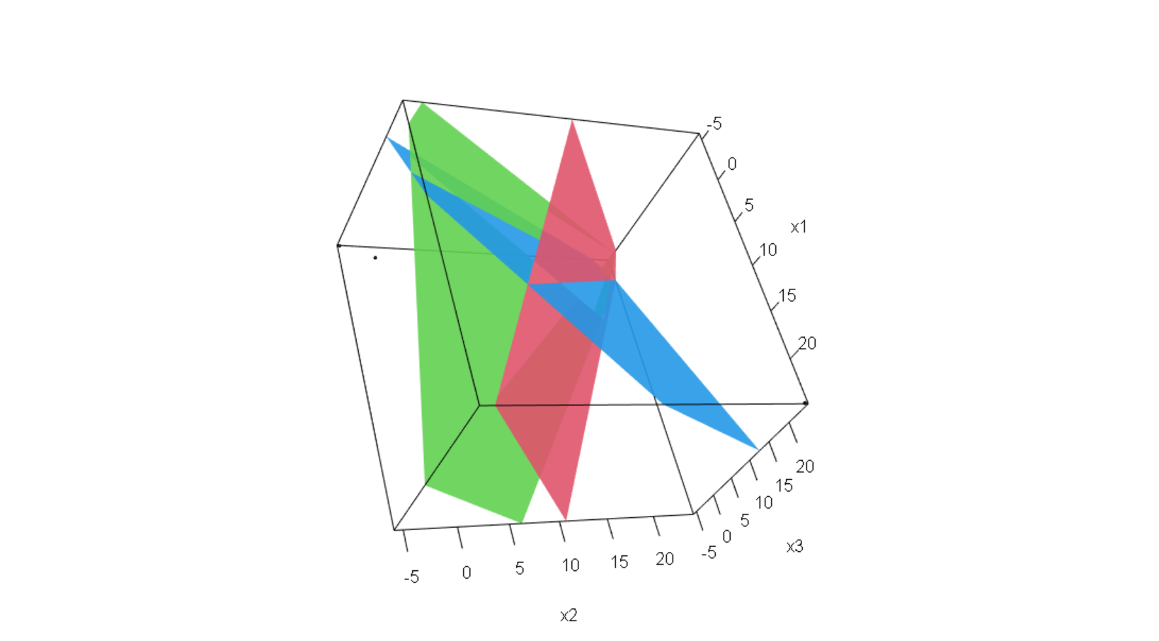

Vector Norm

A norm is a way to measure the size of a vector, a matrix. In other words, norms are a class of functions that enable us to quantify the magnitude of a vector.

Given a \(\text{n-dimensional}\) vector \(\mathbf{X}=\left[\begin{array}{c}x_{1} \\x_{2} \\\vdots \\x_{n}\end{array}\right]\) a general vector norm written with a double bar as, \(\mathbf{||X||}\) is a non-negative norm defined such that,

1. \(||\mathbf{X}||>0\) when \(x \not= 0\) and \(\mathbf{|x|=0 \iff x=0}\).

2. \(|k\mathbf{X}|=|k|\mathbf{|X|}\) for any scalar \(k\).

3. \(\mathbf{||X+Y|| \le ||X|+|Y||}\).

In this case, a single bar is used to denote a vector norm, absolute value, or complex modulus, while a double bar is reserved for denoting a matrix norm.

The matrix norm \(\mathbf{||X||_p}\) for \(p=1, 2, …\) is defined as,

\[ \mathbf{||X||}_p = \Biggl(\sum_{i=1}^n ||x_i||^p\Biggl)^{1/p} \; where \; p>0 \]

This is the defination of \(L^p\)- norm. From this definition one can develop the notion of \(L^1, L^2, \ldots ,L^{\infty}\) norms.

Note:

The subject of norms comes up on many occasions in the context of machine learning:

• When defining loss functions, i.e., the distance between the actual and predicted values

• As a regularization method in machine learning, e.g., ridge and lasso regularization methods.

• Even algorithms like SVM use the concept of the norm to calculate the distance between the discriminant and each support-vector.

Pseudo code of \(L^p\)-norm:

function calculateLpNorm(vector, p):
    // vector is an array representing the vector (x1, x2, ..., xn)
    // p is the parameter for the norm calculation

    if p < 1:
        throw "Invalid value for p. p must be greater than or equal to 1."

    sum = 0

    for i from 1 to length(vector):
        sum += absolute(vector[i])^p

    norm = sum^(1/p)

    return norm

lpNorm <- function(A, p) {
    if (p >= 1 & dim(A)[[2]] == 1 && is.infinite(p) == FALSE) {
            sum((apply(X = A, MARGIN = 1, FUN = abs)) ** p) ** (1 / p)
        
    } else if (p >= 1 & dim(A)[[2]] == 1 & is.infinite(p)) {
        max(apply(X = A, MARGIN = 1, FUN = abs)) # Max Norm
    } else {
        invisible(NULL)
    }
}

lpNorm(A = matrix(data = 1:10), p = 1) # Manhattan Norm

[1] 55

lpNorm(A = matrix(data = 1:10), p = 2) # Euclidean Distance 

[1] 19.62142

lpNorm(A = matrix(data = 1:10), p = 3)

[1] 14.46245

See Also

Inner product for datasets with vector scale (R Documentation)

Outer Product of Arrays (R Documentation)

References

1. Hands-on Matrix Algebra Using R (Active and Motivated Learning with Applications) By Hrishikesh D. Vinod.

2. Basics of Matrix Algebra for Statistics with R By Nick Fieller