It is a truth very certain that when it is not in our power to determine what is true we ought to follow what is most probable.
The Game of Chances
Curiosity is essential to being human from the dawn of humanity. We looked up at the stars and wondered about the universe around us. We have always needed to understand why are things the way they are, where we come from, and what lies ahead. The biggest and most interesting thing i.e., how does the whole universe work, how is arrangement together, was this the clockwork behind it that makes it run the way it does? For thousands of years, we have devised models and principles to explain the world we see around us and the world we cannot see. We are who we are because of the questions we have asked the world because of the answer we have found. But the thing which we have not realized is that whatever phenomenon is taking place in our universe, even in the case of our daily life is uncertain. We do not know when and where our end is. Uncertainty is the biggest mysterious phenomenon in our universe and we do not understand exactly what it is. There is a game that is kept going on always. This is called ‘The game of chances’. There is a strange phenomenon where deterministic & indeterministic processes are kept going on. From this point of view, a new concept or term popped up which is called ‘Probability’ where our goal is to understand the pattern in chaos.
Language to Express Degrees of Beliefs
Probability has evolved from a philosophical background as well as a realistic background. It is an abstract representation of reality. We know that in probability problems, our liability is random. Probability is the language for expressing our degrees of beliefs or uncertainties about any event. Belief systems are ways of thinking that engender specific beliefs. No matter what things one is believing, others will believe different things. Just like religion and politics things diverge, opposing and often antagonizing.
Why such confusion?
Concept of Wishful Thinking
We like to think that we are rational and that what we believe is true. But beliefs conflict. So, who is rational, and who is not? We believe often because of our belief systems. How we believe may be more important than what we believe. Whenever we observe a piece of new evidence, we acquire information that may affect our uncertainties. A new observation that is consistent with an existing belief could make us surer of that particular belief, while a surprising observation could throw that belief into question: how should we update our beliefs in light of the evidence we observe?
Here comes the idea of conditioning which refers to ‘Wishful Think’ i.e., what we wish we knew.
Soul of Probability
Suppose, on a cloudy day you are going out in an overcast condition then you may have to choose whether you will carry an umbrella or not. And that is the valid problem, what you wish you knew. You wish you knew how much it will rain i.e., what you wish you knew. It means that what are the chances that whether the rain will be heavy or not, whether the overcast condition will be clear as the day progress. So, these are kinds of factors that you wish you knew while deciding on carrying an umbrella or not.
Conditioning is a very powerful problem-solving strategy, often making it possible to solve a complicated problem by decomposing it into manageable pieces with case-by-case reasoning. This idea of conditioning applies to solving the complicated problems of probability theory. In probability, a common strategy is to reduce a complicated probability problem to a bunch of simpler conditional probability problems. Conditional probability focuses on how to incorporate evidence into our understanding of the world in a logical, coherent manner. A usual perspective is that all probabilities are conditional; whether or not written explicitly, there is always background knowledge built into every possibility. Rather we update the beliefs to reflect the evidence and as a problem-solving strategy, we say that “Conditioning is the soul of Probability and Statistics”.
Developing Mathematical Guess
Say the probability of getting dengue fever while visiting the Amazon Rainforest for a week is 1 in 10,000 or 0.01%. You go to Amazon Rainforest to come home, and to be safe, take a test that is 99.9% accurate in detecting the virus. Your test comes back positive. You start to freak out, saying goodbye to loved ones, writing out your will, and are about to adopt new religion when you take a second Bayesian look at the results. Remember for every one person with the virus, there are 9,999 people without it, which means that even a robot programmed to always spit out a negative test result, regardless of who’s taking the test, would still guess correctly 99.99% of the time. Being accurate 99.9% of the time, then isn’t really that impressive? what you need to figure out is how accurate that test is when it spits out a positive result. When this one person with the virus takes a test, chances are 99.9% that it will be accurate. Out of the 9,999 people without the virus taking the test, 99.9% of them will get an accurate test result, which translates to 9,989 people. That means that the remaining 10 people will be inaccurately diagnosed, testing positive for dengue fever when they don’t have it. So out of the 11 people testing positive for the dengue virus, only 1 of them has it. It means that the chances your positive test result is right are only 1 in 11, or 9%, not 99.9%.
Now swap dengue fever with HIV, and you are looking at an actual, real-life example have found itself. In case we take the help of conditioning rather Conditional Probability works pretty well and can save your life too.
Early Story
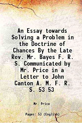
In the early 18th century, Thomas Bayes, the English Nonconformist theologian, mathematician, and Presbyterian minister was the first to use probability inductively and who established a mathematical basis for probability (Generally, calculating from the frequency with which an event has occurred in prior trials, the probability that it will occur in future trials). Bayes set out his theory of probability in “Essay towards solving a problem in the Doctrine of Chances” published in the Philosophical Transactions of the Royal Society of London in 1764. The paper was sent to the Royal Society by Richard Price, a friend of Bayes’, who wrote,
I now send you an essay which I have found among the papers of our deceased friend Mr. Bayes, and which, in my opinion, has great merit… In an introduction he has written to this Essay, he says that his design at first in thinking on the subject of it was, to find out a method by which we might judge concerning the probability that an event has to happen, in given circumstances, upon the supposition that we know nothing concerning it but that, under the same circumstances, it has happened a certain number of times, and failed a certain other numbers of times.
Way to Begin
While Ben Franklin is running around flying kites, Thomas Bayes is figuring out how to make educated mathematical guesses in situations where you do not have that much to go on, like possibly the probability that a guy name ‘X’ exists. But then Bayes dies before He is having a chance to tell anyone what he’s been up to. Soon after, his philosopher buddy, Richard Price, discovers Bayes’ notebooks while digging around his apartment, looking for free swag. Price is a pretty smart guy, so he instantly recognizes the genius of his pal’s theory. In 1763, he cleans up the math and publishes it in an obscure journal before using it to revolutionize the insurance business, where they need probabilities to figure out how much to rip you off. Fast forward to 1812, while the US and England are at it again, a French guy named Pierre-Simon Laplace developed Bayes’ theory into something more usable, which becomes known as conditional probability. It lets you update your guesses with any new facts that might come your way.
Towards The Bayesian Paradigm
That work became the basis of a statistical technique, now called Bayesian Estimation, for calculating the probability of the validity of a proposition based on a prior estimate of its probability and new relevant evidence. Bayes never used the phrase Bayesian analysis. He published only two papers in his life, one theological and one in which he defended Newton’s calculus against criticism from philosopher George Berkeley. But late in life, Bayes became interested in probability. He died in 1761, and a year after his death his friend Richard Price arranged for a public reading of a paper by Bayes in which he proposed what became known as Bayes’ Theorem. His formula prescribed how one could update initial beliefs about an event with information from data.
The goal of this article is to unfold the insight of one of the most important formulas in all of probability, Bayes’ Theorem. This formula is central to scientific discovery, it’s a core tool in statistics, machine learning, and information theory. It’s even been used for treasure hunting, when in the 80’s a small team led by Tommy Thomson used Bayesian search theory to help uncover a ship that had sunk a century earlier carrying what, in today’s terms, amounts to \(700 \; \text{M}\) worth of gold.
A Bayesian Approach To Finding Lost Objects
A Speck in the Sea
In 2014 a man named John Aldridge was working on a lobster boat. He was 65 kilometers off the tip of Long Island and it was the middle of the night. But while working a handle that he was using for leverage snapped sending him flying backward into the ocean, he yelled back to the two other people on the boat. But they were sleeping and the engine was too loud so the boat which was on autopilot faded into the night. It was 3:30 in the morning and John was stranded in the Atlantic Ocean with one goal to stay alive. It was not until 6 a.m. when the other two men on board woke up and they immediately called the coast saying they’d got a man overboard. Now they had no idea if he fell off 5 minutes ago or 8 hours ago. All they knew was their current location and the last time they saw him. Based on the water temperature and weather the Coast Guard determined that John had about 19 hours of survival window before hypothermia took over and his muscles gave out. So, now it was a race against the clock to figure out where he was, and here’s what they did.
Strategy Behind Searching
Based on the current position and two autopilot speeds they could determine the maximum distance John could be from that location. From this, we can sweep out a circle
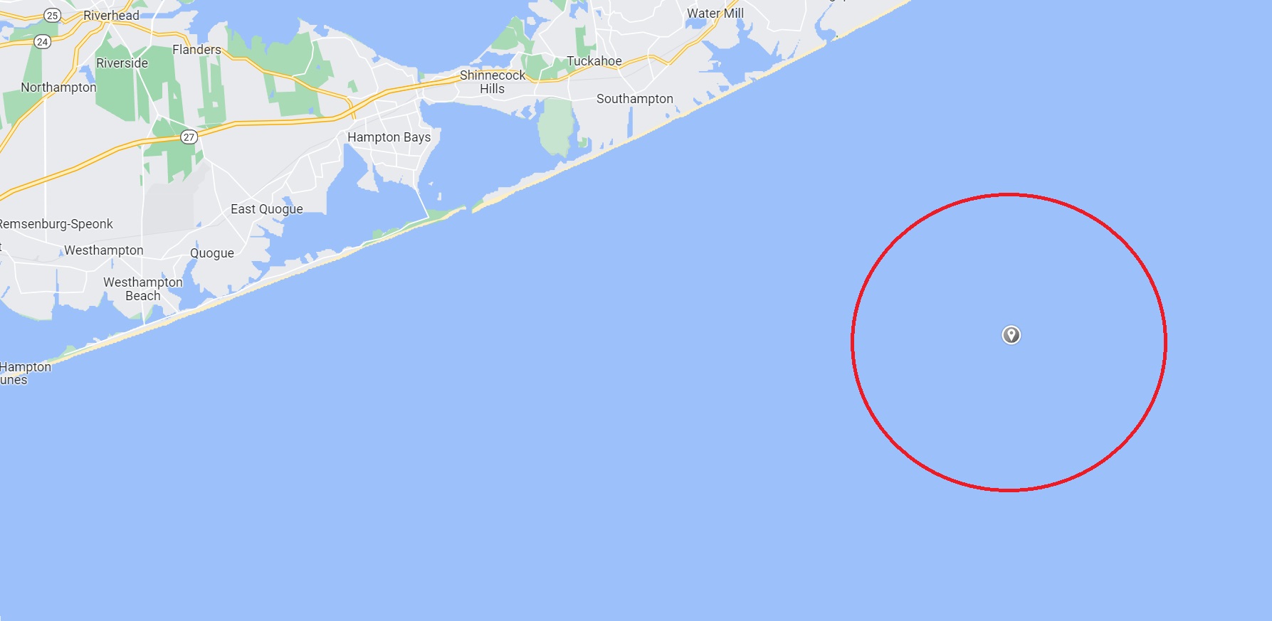
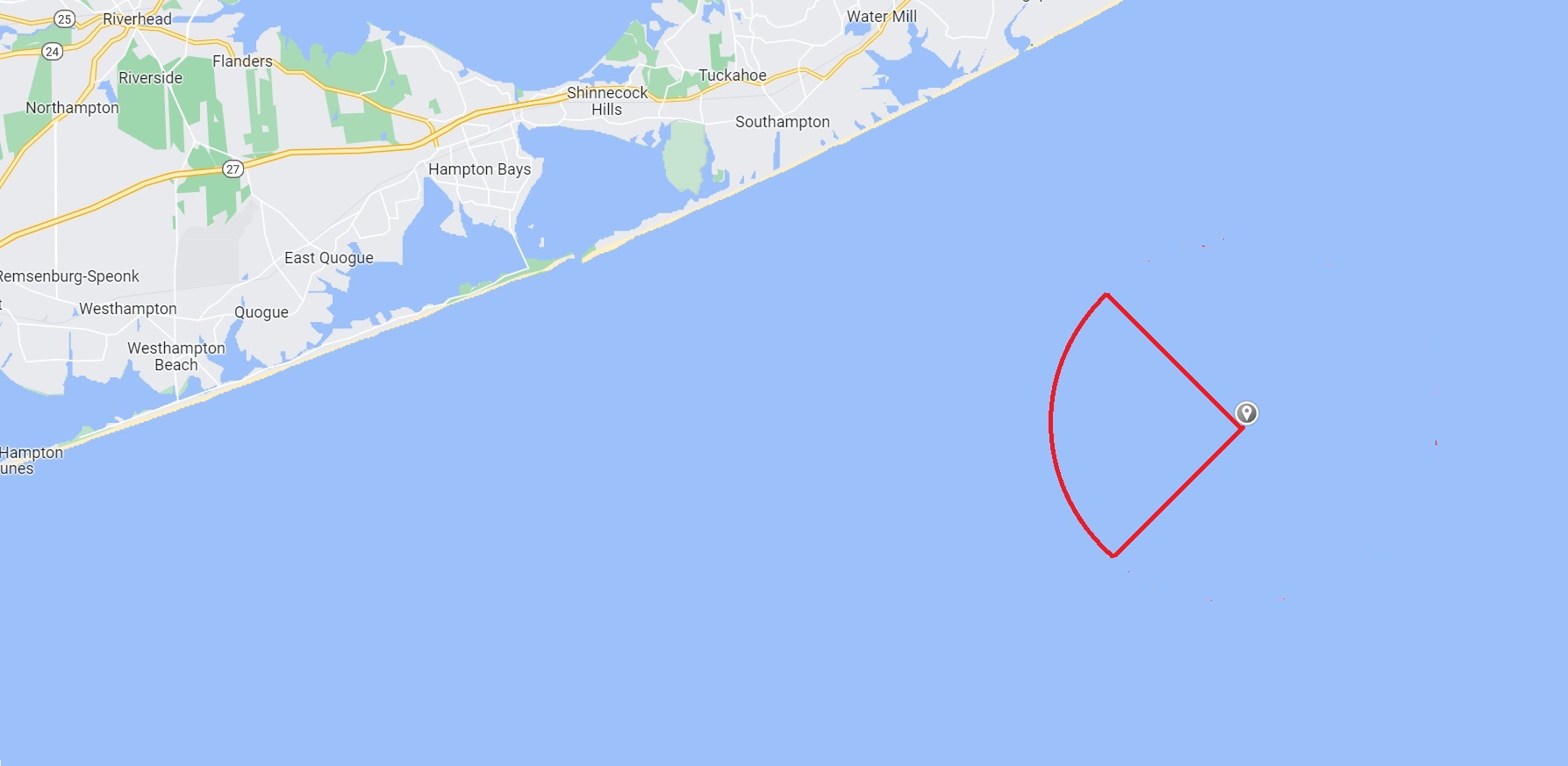
which tells if John stayed put he has to be somewhere in the circle. But the boat was on a course away from the shore, so we could narrow that region down then the Coast Guard input all the given information into something knows the search and rescue optimal planning system which operates based on math, statistics, and actual data about the weather, ocean currents and so on.

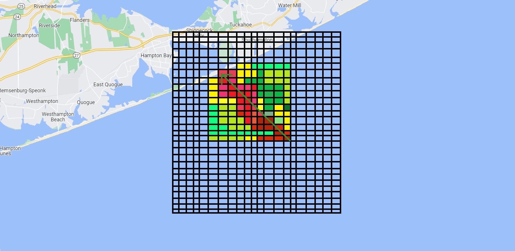
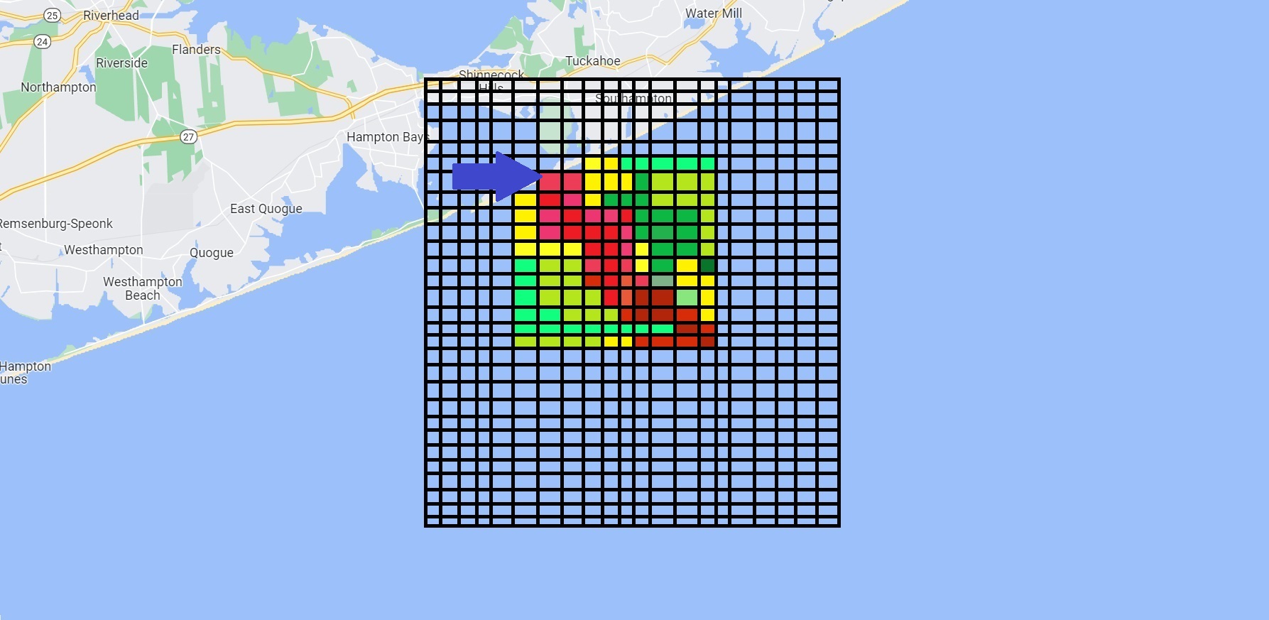
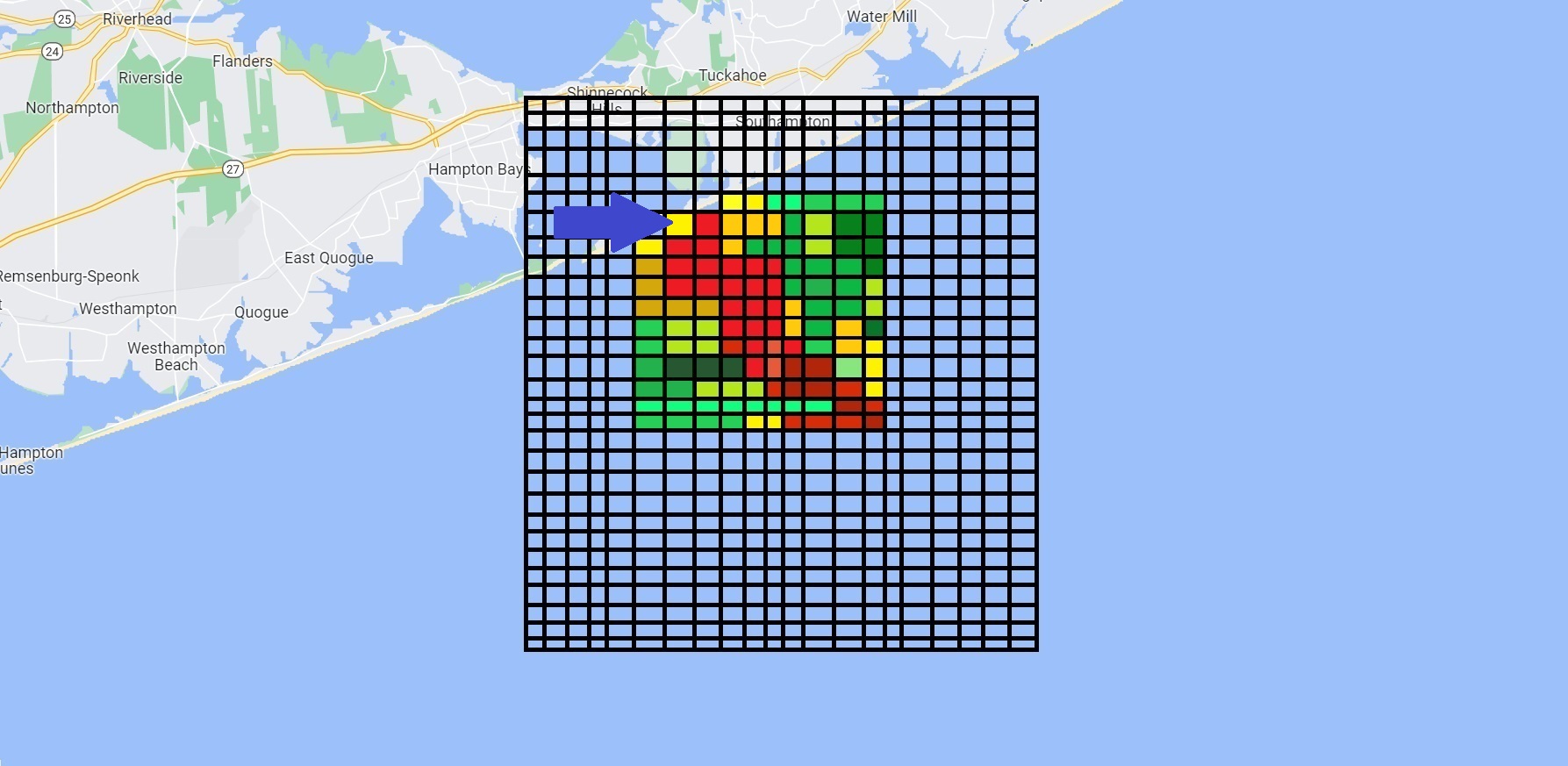
The system superimposes a grid over the ocean and assigns each square a probability that John is there based on given information. Since there were several hour-long periods where he could have fallen out. We could expect to see a long strip of high probabilities and thus the search began.
Imposing Probability Theory
Methodology
According to the picture below if we first search on the blue arrow marked place and don’t find him does that mean he’s not here and thus the new probability is \(0?\) The answer is no. He’s a small head in a huge we could just have missed them.

So, after we search a grid we need to update its probability not just set it to \(0\) and this brings us to Bayesian search theory an application of Bayesian statistics that are used to find lost objects. The foundation of this theory is Bayes’ Theorem. But we’re going to use it to keep things simple either way the goal here is to find the probability of some event \(\text{A}\) being true given that another event \(\text{B}\) is true (which is nothing but \(\text{P(A|B)}\)).
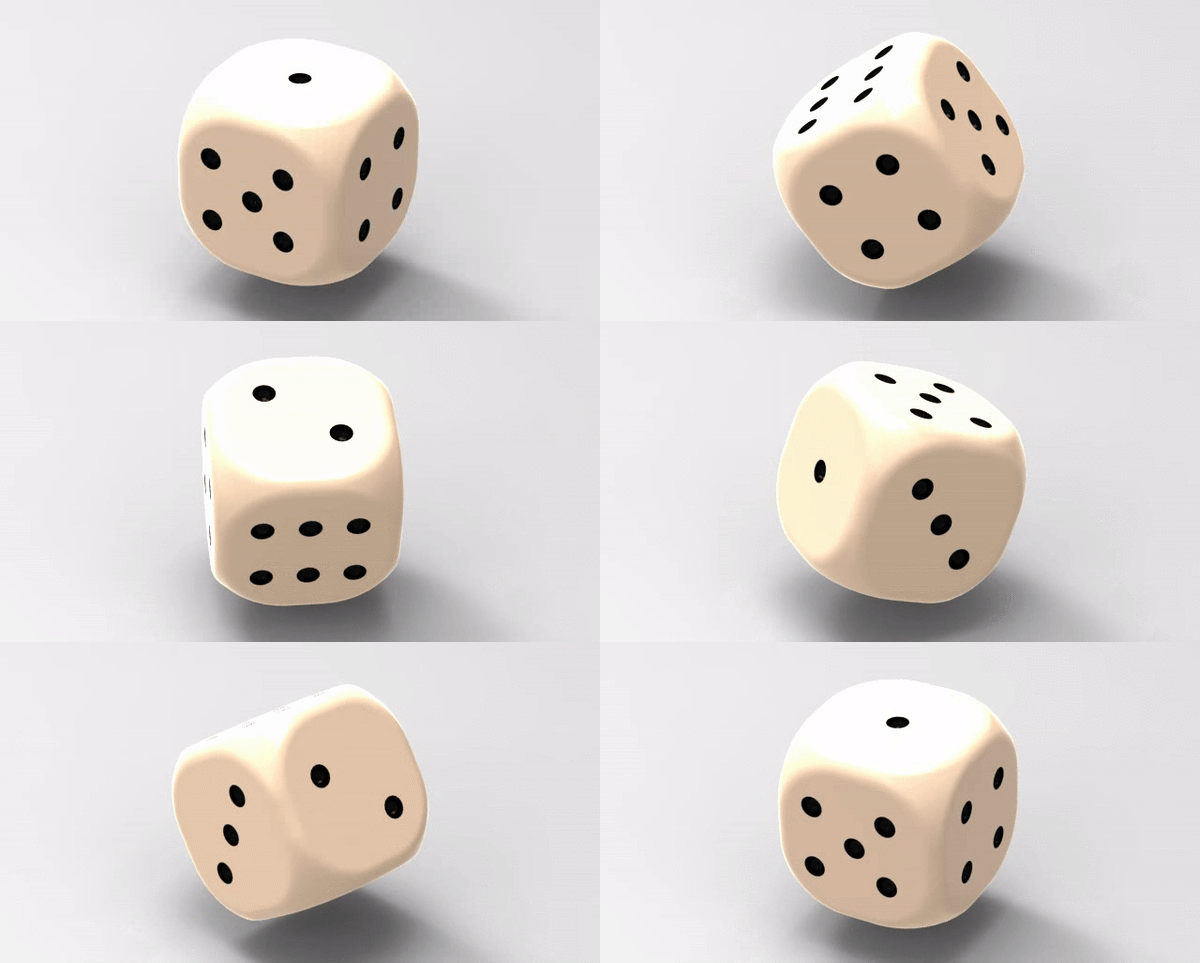
For example, if we roll the die and hid the result from you then ask what’s the chances of \(5?\) You would say \(\text{P}(5) = \frac{1}{6}.\) But, if there is more information provided to you. Like, the rule that came out odd is relevant given that reveals more about the situation. So, the probability of it being a \(5\) given that it’s odd i.e., \(\text{P}(5|\text{Odd}) = \frac{1}{3}.\) New information can change things. Now Bayes’ theorem for the probability of A given B is written as below,
\[\text{P}(\text{A}|\text{B}) = \dfrac{\text{P}(\text{B}|\text{A}) \text{P}(\text{A})}{\text{P}(\text{B})}\]
\(\text{which can be derived from this formula}\; \frac{\text{P}(\text{A}\;\cap\;\text{B})}{\text{P}(\text{B})}.\text{Where the numerator just means the}\) \(\text{probability}\)\(\text{ that both events are true.}\)
Probability Tree
Execution Process
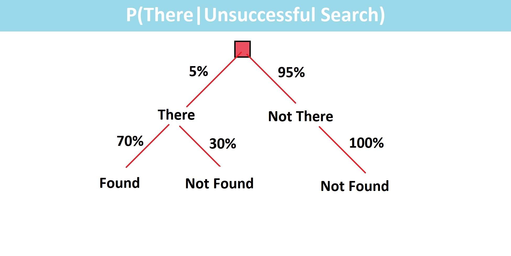
Now, going back let’s say we search for this square and don’t find him. We now want a new probability, the probability that he is there given that we looked and didn’t find him. Well, for that two square, he’s either there or he’s not. Maybe this Square has a \(5\%\) chance that he’s there according to the researcher who computed. If he’s in that square, he will either be found or not. Maybe the skies are clear, so there’s a \(70\%\) chance that you find him if you look, but still, a \(30\%\) chance you miss him. If he is not in the square then of course he won’t be found with \(100\%\) certainty.
Computing The Probability
From the formula of conditional probability, we express \(\text{P}(\text{A}|\text{B})\) as,
\[ \text{P}(\text{A}|\text{B})= \dfrac{\text{P}(\text{A}\cap \text{B})}{\text{P}(\text{B})} \]
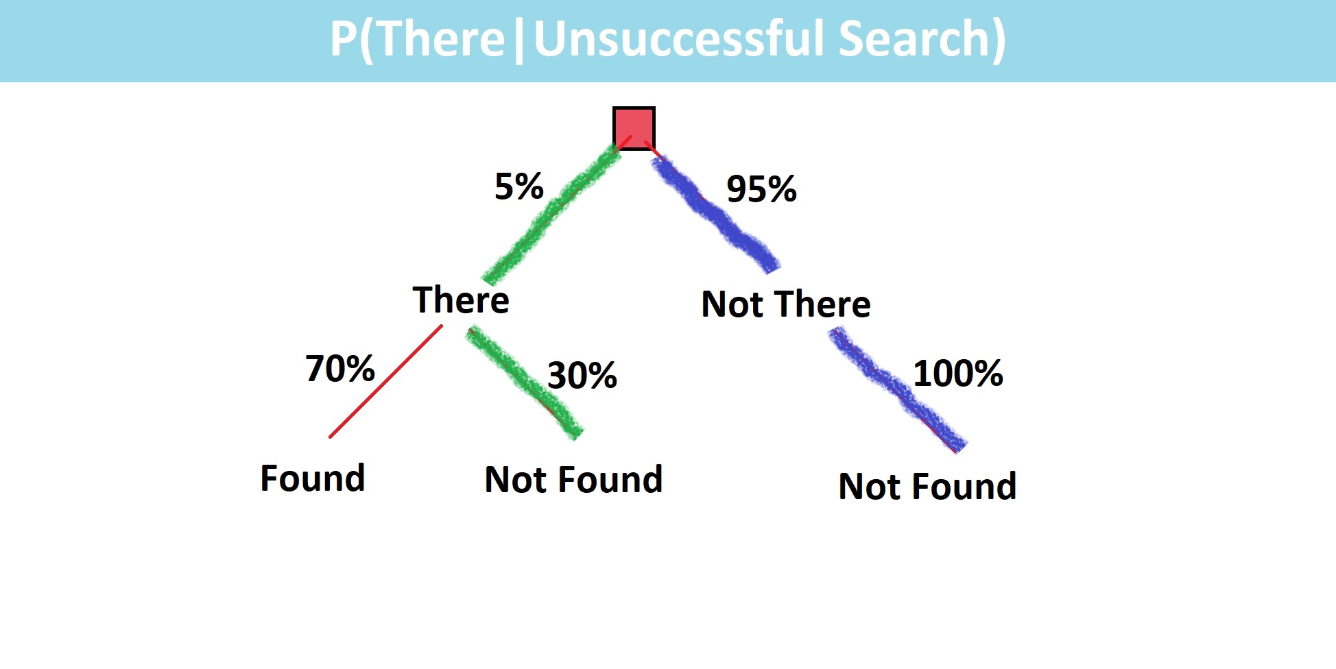
We are first going to find the probability that he is in the square and also not found as those are the two events that we listed up. Here, the probability that he’s in the square and not found can be determined by just going down two green branches and multiplying those probabilities together. Then we need to find the probability that he’s not in that square period which can be determined by going down green & blue two branches that both ends are not found.
\(\text{P}(\text{There|Unsuccessful Search})=\) \(\dfrac{\text{P(There and Not Found)}}{\text{P(Not Found)}}\)
\[ \hspace{1.5 cm}= \dfrac{(0.30)(0.05)}{(0.05)(0.30)+(1)(0.95)} = 1.55\% \]
We add the product of those probabilities and we get a value of about \(1.55\%\) which again is the chance that he is still in that square given that we couldn’t find him there. If we go back to our grid that square we just searched is now updated to its new \(1.55\%\) probability. Since that square went down the other square probabilities go up by a small amount. It’s best to continue

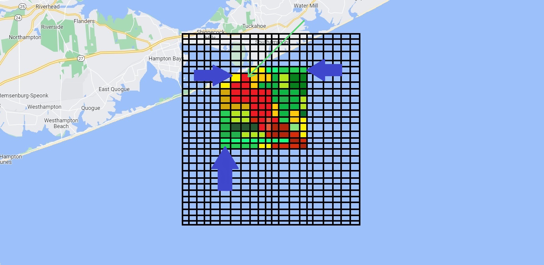
our search probably with the square marked by the green arrow. But after a few hours of searching, we can see it might be more beneficial to search that original search again rather than one of these lower probability green squares out here.
Inverse Cube Law
Now, through various studies a while back it was determined that the probability of detecting an object is inversely related to the cube of the distance away. The constant is determined experimentally based on things like the depth of the water if the object is submerged or the size of the object that you’re looking for.
In search theory, the definite range law, the imperfect definite range law, and the inverse cube law have been used to investigate search problems. In these detection laws, only the inverse cube law is a decreasing function of distance. This law was given by Koopman in his study on search theory during WW II. The detection rate of the inverse cube law is defined by
\[ f(r) = \dfrac{k}{r^3} \]
This is one way that the probability value we saw earlier could be estimated for those who are curious.
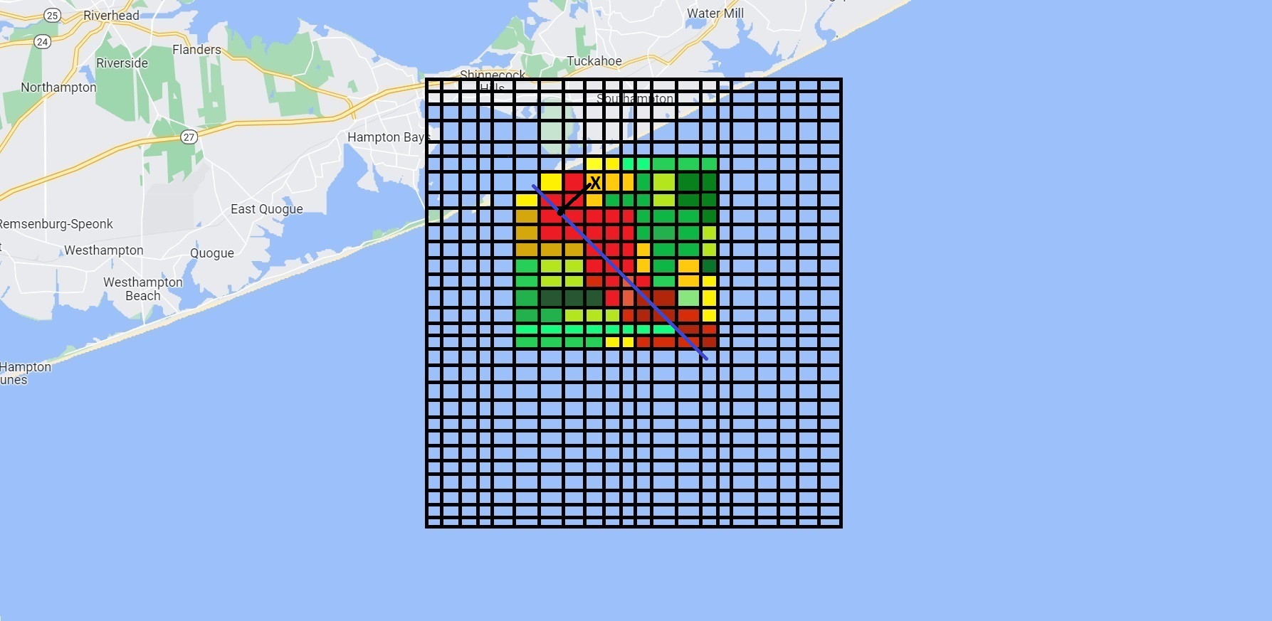
So, if John is at point X and the helicopter flies along this blue straight-line path looking for him at any given point there’s some probability of locating John based on the distance. This probability changes at each point and if we integrate or sum values along the line we get a total probability of detection for that line.
Optimized Search Patterns
Now the problem is we don’t know where John is so we need to just do sweeps that optimize our odds which means we need to apply optimized search patterns.
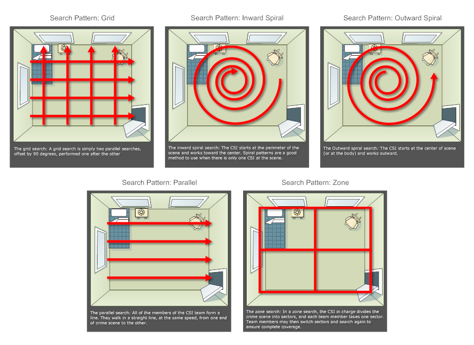
Now if there’s a high probability of John being in one certain location like if we knew exactly where he fell off then an expanding square search might be ideal to cover areas of higher probabilities. Sometimes a creeping line search is better but in this case, it was best to use a parallel search running parallel to the strip of high probability. All these things have been calculated using mathematics, and statistics based on given information.
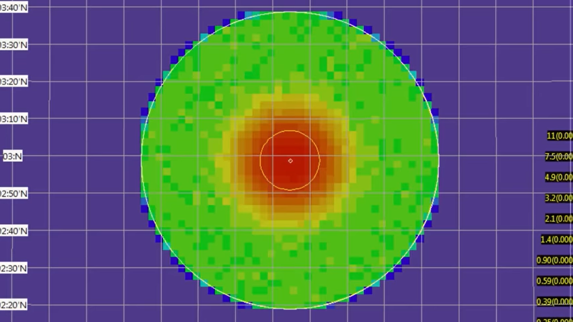
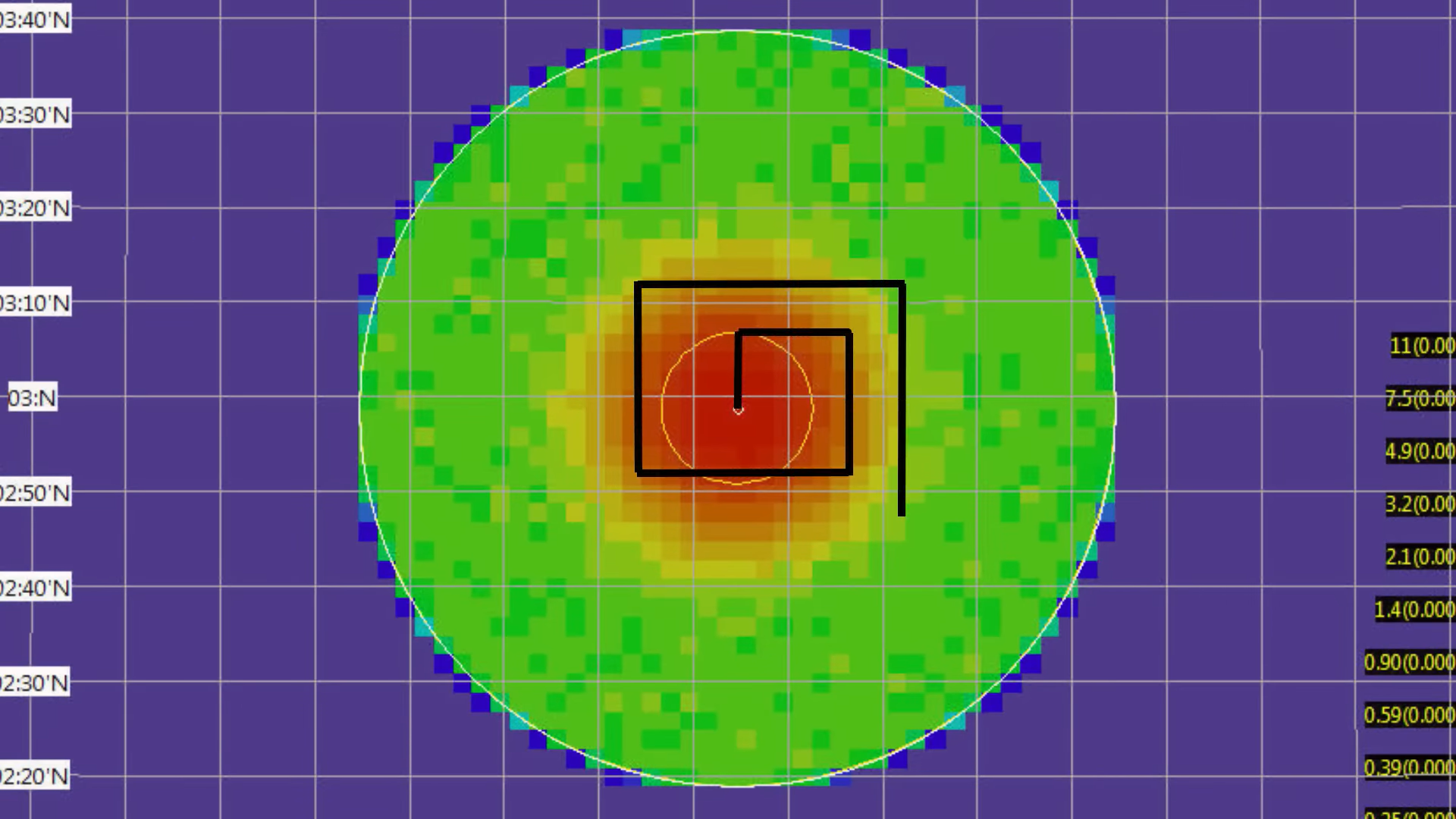
Practically, always going for the square with the maximum probability may not be the most efficient method because you may have to travel all across the area and it might be more efficient to search areas you are traveling through as you go. After the initial probabilities have been found for the area, a search plan will likely be created for your planned search journey. This may not necessarily have you always searching the areas in descending probability order. However, with Bayesian search theory applied you can get a useful indication of where would be wise to search and when to amend your search plan.
Time to Go Home
Now after hours in the water, John managed to find something to keep him afloat but he had lost so much energy he was preparing for the real chance of dying he decided to soon tie his body to the object. So when he was found the body could be delivered to his parents they’d have something to bury. But Finally 3 p.m. on one of the final sweeps the search team saw John and got him safely to the hospital where he was treated for hypothermia and made a full recovery so he could tell the story. Without John’s ability to stay calm at sea and a formula that dates back a few hundred years, likely, this man wouldn’t be alive today.
See Also
References
Introduction to Probability Book by Jessica Hwang and Joseph K. Blitzstein.
Mathematical Statistics by Parimal Mukhopadhyay.
A Philosophical Essay on Probabilities by Pierre-Simon Laplace.
I Hacking, Biography in Dictionary of Scientific Biography (New York 1970-1990).
J P Clero, Thomas Bayes. Essai en vue de résoudre un problème de la doctrine des chances (Paris, 1988).
D A Gillies, Was Bayes a Bayesian?, Historia Math. 14 (4) (1987), 325-346.
Thomas Bayes’s essay towards solving a problem in the doctrine of chances, in E S Pearson and M G Kendall, Studies in the History of Statistics and Probability (London, 1970), 131-153.
S M Stigler, who discovered Bayes’s theorem? The American statistician 37 (1984), 290-296.
A I Dale, Bayes or Laplace? An examination of the origin and early applications of Bayes’ theorem, Arch. Hist. Exact Sci. 27 (1) (1982), 23-47.
J P Clero, Thomas Bayes. Essai en vue de résoudre un problème de la doctrine des chances (Paris, 1988).
INVERSE NTH POWER DETECTION LAW FOR WASHBURN’S LATERAL RANGE CURVE
Washburn,A.R., Search and Detection, Military Applications Section, Operations Research Society of America, 1981.