” An exceptionally potent weapon”
Inequality is an exceptionally potent weapon. There are many occasions on which persons who know and think of using this formula can shine while less fortunate brethren flounder
Towards Cauchy-Schwarz
An argument can be drawn based on both analytic geometry and complex numbers to derive one of the most useful tools in the analysis \(-\)the so-called Cauchy-Schwarz inequality. We are going to explore an amusing example, of how inequality can squeeze a solution out of what seems to be nothing more than a vacuum.
If \(f(t)\) and \(g(t)\) are any two real-valued functions of the real variable \(t\), then it is certainly true, for \(\lambda\) any real constant, and \(U\) and \(L\) two more constants (either or both of which may be arbitrarily large, i.e., infinite), that
\[\int_{L}^U[ f(t)+\lambda g(t)]^2 dt \ge0\\\]
\[\implies \lambda^2 \int_{L}^U g^2(t)\ dt\ + \ 2\lambda \int_{L}^U f(t)\ g(t)\ dt\ + \ \int_{L}^U f^2(t)\ dt \ge 0 \]
This is so because, as something real and squared, the integrand is nowhere negative. We can expand the integral. Since these three definite integrals are constants(call their values a,b, and c) we have the left-hand side as simply a quadratic in \(\lambda\), \[h(\lambda)=a\lambda^2+ 2b\lambda+c \ \ge0\ \]
Where,
\[a= \int_{L}^U g^2(t)\ dt, \ b= \int_{L}^U f(t)\ g(t)\ dt ,\ d=\int_{L}^U f^2(t)\ dt \]
The inequality has a simple geometric interpretation: a plot of \(h(\lambda)\) versus \(\lambda\) cannot cross the \(\lambda\) -axis.
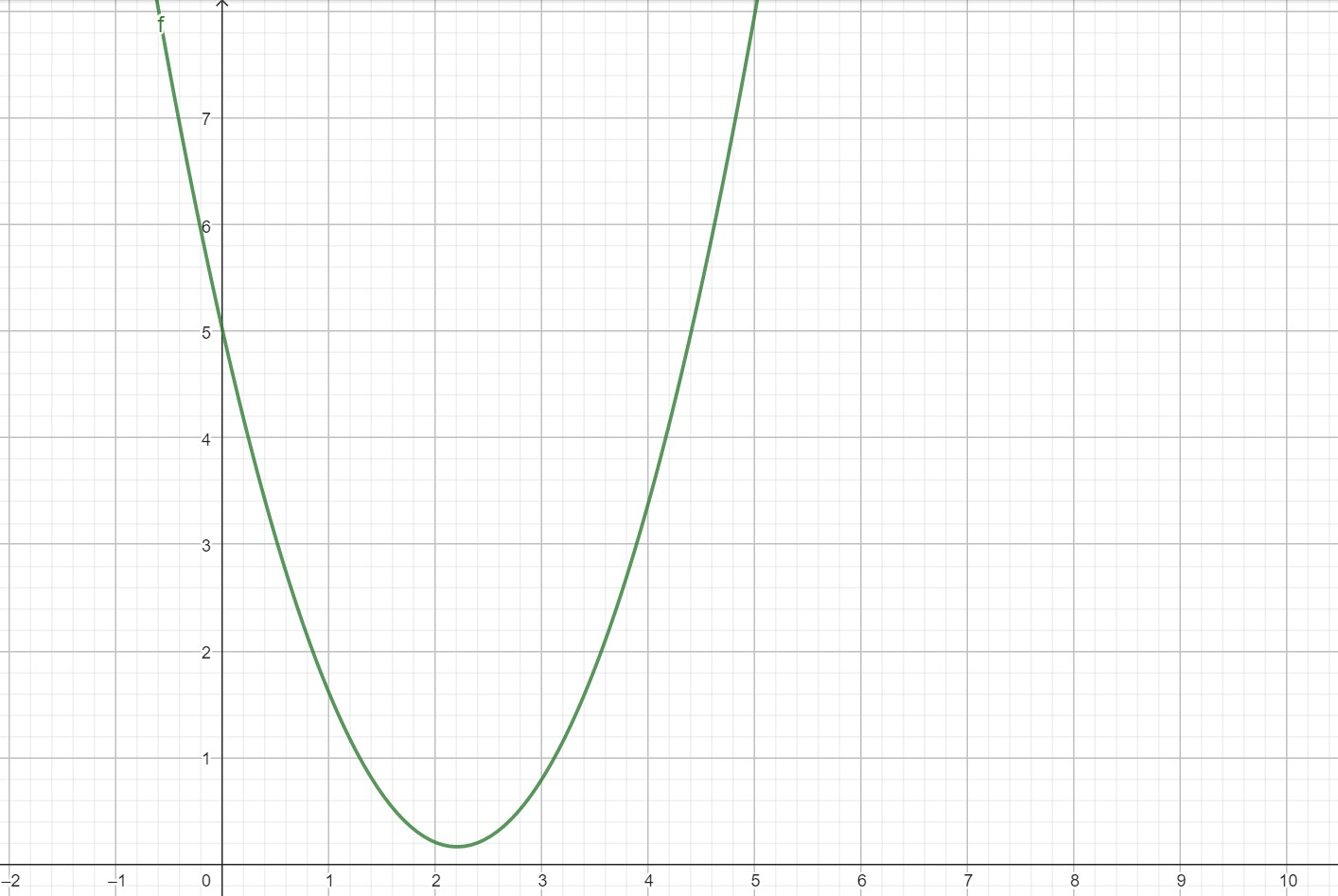
At most that plot (a parabolic curve) may just touch the \(\lambda\) - axis, allowing the ” greater-than-or-equal to” condition to collapse to the special case of strict equality, i.e., to \(h(\lambda)=0\), in which the \(\lambda\) - axis is the horizontal tangent to the parabola. This, in turn, means that there can be no real solutions ( other than a double root ) to \(a\lambda^2+ 2b\lambda+c=0\) , because a real solution is the location of a \(\lambda\) - axis crossing. That is, the two solutions to the quadratic must be the complex conjugate pair
\[\lambda= \dfrac{-2b\pm\sqrt{4b^2-4ac}}{2a}=\dfrac{-b\pm\sqrt{b^2-4ac}}{a}\]
where, of course, \(b^2\le ac\) is the condition that gives complex values to \(\lambda\) ( or a real double root if \(b^2-ac=0\) ). Thus our inequality \(h(\lambda) \ge 0\) requires that
\[ \bigg\{\int_L^U f(t)g(t)dt \bigg\}^2 \le \bigg\{\int_L^U f(t)^2dt \bigg\} \bigg\{\int_L^U g(t)^2dt \bigg\} \]
and we have the Cauchy-Schwarz inequality.
Mathematical Problem
As a simple example of the power of this result, consider the lowing. Suppose, a man climbs to the top of a 400-foot-high tower and then drops a rock. Suppose further that we agree to ignore such complicating “little” details as air drag. Then, as Galileo discovered centuries ago if we call \(y(t)\) the distance the rock has fallen downward toward the ground (from that man’s hand), where \(t=0\) is the instant the man let go of the rock and if \(g\) is the acceleration of gravity (about \(32\ ft/sec^2\)), then the speed of the falling rock is \(v(t)=\dfrac{dy}{dt}=gt=32t\ ft/sec)\) (measuring time seconds). So (with \(s\) a dummy variable of integration)
\[y(t)=\int_0^tv(s)\ ds\]
\[=\int_0^t32s\ ds\]
\[= (16s^2|_0^t=16t^2\]
If the rock hits the ground at time \(t=T\), then \(400=16T^2\) or \(T=5\) sec.
With this done, it now seems to be a trivial task to answer the following question:
What was the rock’s average speed during its fall? Since it took five seconds to fall 400 feet, then we can suspect 9,999 out of 10,000 people would reply “Simple. It’s 400 feet divided by 5 seconds or 80 feet/second.” But what would that 10,000 person say, you may wonder? Just this: what we just calculated is called the time average
i.e.,
\[ V_{time}=\dfrac{1}{T}\int_0^T v(t)\ dt \]
That is, the integral is the total area under the \(v(t)\) curve from \(t=0\) to \(t=T\), and if we imagine a constant speed \(V_{time}\) from \(t=0\) to \(t=T\) bounding the same area (as a rectangle, with \(V_{time}\) as the constant height), then we have the above expression. And, indeed, since \(v(t) = 32t\), we have
\[ V_{time}=\dfrac{1}{5}\int_{0}^{5}32t\ dt= \dfrac{32}{5} \bigg[\dfrac{t^2}{2}\bigg]_0^5=80 \ ft/sec \]
just we originally found.
And then, as we all nod in agreement with this sophisticated way of demonstrating what was “obviously so” from the very start, our odd-man-out butts in to say
“But there is another way to calculate an average speed for the rock, and it gives a different result!”
Instead of looking at the falling rock in the time domain, he says, let’s watch it in the space domain. That is, rather than speaking of \(v(t)\), the speed of the rock as a function of the time it has fallen, let’s speak of \(v(y)\), the speed of the rock as a function of the distance it has fallen. In either case, of course, the units are \(ft/sec\). If the total distance of the fall is \(L\) (400 feet in our example), then we can talk of a spatial average,
\[ V_{space} = \dfrac{1}{L}\int_{0}^{L} v(y)\ dy \] Since \(t=\sqrt{\dfrac{y}{16}}=\dfrac{1}{4}\sqrt{y}\) , then \(v(y)=32\bigg(\dfrac{1}{4}\sqrt{y}\bigg)=8\sqrt{y}\). When \(y=400ft\), for example, this says that \(v(400)=8\sqrt{400}=160ft/sec\) at the end of the fall, which agrees with our earlier calculation of \(v(5)=160ft/sec\). Thus, our falling rock,
\[V_{space}=\dfrac{1}{400}\int_0^{400}8\sqrt{y}\ dy\]
\[ =\dfrac{1}{50}\bigg[\dfrac{2}{3}y^{\frac{3}{2}}\bigg]_0^{400} \]
\[= \dfrac{1}{75}.\ 400^{\dfrac{3}{2}} \approx 107ft/sec\]
We could discuss, probably for quite a while, just what this result means, but all we want to do here is to point out that \(V_{time}\le V_{space}\). In fact, although we have so far analyzed only a very specific problem, it can be shown that no matter how \(v(t)\) varies with \(t\) (no matter how \(v(y)\) varies with \(y\)), even if we take into account the air drag we neglected before,\(V_{time}\le V_{space}\) . This is a very general claim, of course, and there is a beautiful way to show its truth using the Cauchy-Schwarz inequality (which, of course, is the whole point of this section!) Here’s how it goes.
\(Let\ g(t) = \dfrac{v(t)}{T} \ and \ f(t) = 1.\)
Then the Cauchy-Schwarz inequality says,
\[ \bigg(\dfrac{1}{T}\int_0^Tv(t)dt\bigg)^2 \le\ \bigg\{\int_0^T dt\bigg\}\ \bigg\{\dfrac{1}{T^2}\int_0^T v^2(t)dt \bigg\} \]
\[= \dfrac{1}{T} \int_0^T v^2(t)dt\]
\[ = \dfrac{1}{T} \int_0^T \bigg(\dfrac{dy}{dt}\bigg)^2 dt \]
Now, taking advantage of the suggestive nature of differential notation,
\[\bigg(\dfrac{dy}{dt}\bigg)^2 dt= \dfrac{dy}{dt}.\ \dfrac{dy}{dt}.\ dt =\dfrac{dy}{dt}.dy\]
If we insert this into the last integral above, then we must change the limits on the integral to be consistent with the variable of integration, that is, with \(y\). Since \(y=0\), \(t=0\), and \(y=L\), \(t=T\). Then we have,
\[\bigg(\dfrac{1}{T}\int_0^Tv(t)dt\bigg)^2 \le \ \dfrac{1}{T}\int_0^L \dfrac{dy}{dt}\ dy\]
\[\ \ \ \ = \dfrac{1}{T} \int_{0}^{L} v(y)\ dy\]
\(Now,\ L= \int_0^Tv(t)\ dt, \ and \ so\)
\[\bigg\{\dfrac{1}{T}\int_0^Tv(t)dt\bigg\}\bigg\{\dfrac{1} {T}\int_0^Tv(t)dt\bigg\} = \bigg(\dfrac{1}{T}\int_0^Tv(t)dt\bigg)\dfrac{L}{T}\]
\[\hspace{4cm}\le \dfrac{1}{T} \int_{0}^{L} v(y)\ dy\]
\(Thus,\)
\[ \dfrac{1}{T} \int_{0}^{T} v(t)\ dt \le \dfrac{1}{L} \int_{0}^{L} v(y)\ dy \]
\(and \ so\ \ V_{time}\le V_{space}\) as claimed, and we are done.
A Generic Conclusion
Nowhere in the above analysis we have made any assumptions about the details of either \(v(t)\) or \(v(y)\), and so our result is completely general. This result would be substantially more difficult to derive without the Cauchy-Schwarz inequality, and so don’t forget how we got it with arguments that depend in a central way on the concept of complex numbers.
References
Kadison, R. V. (1952), “A generalized Schwarz inequality and algebraic invariants for operator algebras”, Annals of Mathematics, 56 (3): 494–503, doi:10.2307/1969657, JSTOR 1969657.