Chaos and Butterfly Effect

The scientific theory that a single occurrence, no matter how small, can change the course of the universe forever

INTRODUCTION

Dynamical systems theory is an area of mathematics i.e., used to describe the behavior of complex dynamical systems, usually by employing differential equations or difference equations. When differential equations are employed, the theory is called continuous dynamical systems. From a physical point of view, continuous dynamical systems are a generalization of classical mechanics, a generalization where the equations of motion are postulated directly and are not constrained to be Euler–Lagrange equations of a least action principle. When difference equations are employed, the theory is called discrete dynamical systems. When the time variable runs over a set that is discrete over some intervals and continuous over other intervals or is any arbitrary time set such as a Cantor set, one gets dynamic equations on time scales. Some situations may also be modeled by mixed operators, such as differential-difference equations.

This theory deals with the long-term qualitative behavior of dynamical systems, and studies the nature and when possible the solutions of the equations of motion of systems that are often primarily mechanical or otherwise physical, such as planetary orbits and the behavior of electronic circuits, as well as systems that arise in biology, economics, and elsewhere. Much of modern research is focused on the study of chaotic systems.

CHAOS THEORY

Chaos theory is a branch of mathematics focusing on the study of chaotic dynamical systems whose random states of disorder and irregularities are governed by underlying patterns and deterministic laws that are highly sensitive to initial conditions. Chaos theory is an interdisciplinary theory stating that, within the apparent randomness of chaotic complex systems, there are underlying patterns, interconnectedness, constant feedback loops, repetition, self-similarity, fractals, and self-organization. The butterfly effect, an underlying principle of chaos, describes how a small change in one state of a deterministic nonlinear system can result in large differences in a later state (meaning that there is a sensitive dependence on initial conditions). Small differences in initial conditions, such as those due to errors in measurements or due to rounding errors in numerical computation, can yield widely diverging outcomes for such dynamical systems, rendering long-term prediction of their behavior impossible in general. This can happen even though these systems are deterministic, meaning that their future behavior follows a unique evolution and is fully determined by their initial conditions, with no random elements involved. In other words, the deterministic nature of these systems does not make them predictable. This behavior is known as deterministic chaos, or simply chaos. The theory was summarized by Edward Lorenz as Chaotic behavior exists in many natural systems, including fluid flow, heartbeat irregularities, weather, and climate. It also occurs spontaneously in some systems with artificial components, such as the stock market and road traffic. This behavior can be studied through the analysis of a chaotic mathematical model, or analytical techniques such as recurrence plots and Poincare maps. Chaos theory has applications in a variety of disciplines, including meteorology, anthropology, sociology, failed verification environmental science, computer science, engineering, economics, ecology, pandemic crisis management, and philosophy. The theory formed the basis for such fields of study as complex dynamical systems, edge of chaos theory, and self-assembly processes.

LORENTZ SYSTEM

At The Beginning of The Revolution

In August 2017, people across North America planned for a once-in-a-lifetime opportunity to watch a total solar eclipse. Here’s a reference to the 2017 eclipse in an article about a previous one, 99 years earlier.

Reference to the 2017 eclipse in an article

For centuries, humans have used math and science to make predictions about our universe. Certainly, by the end of the 19th century, scientists felt that we were living in a Cartesian universe, in which, if you had some omniscient being who knew the positions and velocities of all the particles in the universe, in principle, that being would know what would happen for all time.

Greek Eclipse Calculator ( about 100 BC )

But if that’s true, why are some things in our world still so hard to predict, even in an era of supercomputers and big data? If we can predict an eclipse a century in advance, why can we only predict the weather about a week or two in advance?

Mayan Eclipse Table ( About 1200 AD )

We know this system is based on the same physical laws as the rest of our universe, but it seems random. The study of systems that look random, but aren’t, is called ” Chaos Theory”, one of its key pioneers was an MIT meteorologist named Edward Norton Lorenz. During World War II and the decades that followed, Computers allowed scientists to take major steps forward in weather prediction.

Experiments and Results

In 1961, Lorenz was working with a set of equations that represented a simplified version of the atmosphere, with 12 variables that changed over time. The computer calculated the values for each moment in time by applying the equations to the values from the previous moment, and Lorenz watched how they progressed. He needed to be sure that like real weather, they did not follow a repeating pattern. In, some cases, Lorenz’s team needed to reprint part of the simulation, so they would restart it from an earlier point by entering the numbers from an earlier printout as start values. Since they used the same numbers and equations, they expected to see the same results.

But sometimes they didn’t. In some cases, the second run would look very different from the first as it progressed. At first, Lorenz thought the computer was malfunctioning, but he eventually found the source of the error. While the computer’s memory stores numbers with six decimal places, it printed them with only three decimal places, so the values he entered contained tiny errors.

Lorenz was observing that in some systems, tiny changes in the present can lead to big changes in the future. 

Courtesy of Glenn Flierl & Lodovica Illri( MIT )

Today we can create models of the atmosphere that go far beyond Lorenz’s columns of numbers. In this model from MIT, the white line represent a bunch of balloons released from approximately the same point. Eventually, the Balloons diverge along very different paths, because of the small differences in their starting points. If you change the initial conditions ever so slightly, infinitesimally slightly. The two trajectories seem to go along with each other and then they diverge exponentially fast. So, that is chaos. It means that you have to know a system with infinite precision to be able to predict it infinitely in time. 

Sensitive Dependence on Initial Conditions

In 1903, French mathematician Henri Poincare observed something similar while studying the problem of three objects in space, all affected by each other’s gravity. He was always looking for what’s the most simple set of equations that exhibit chaotic properties. Lorenz found a set of three equations, a simplified version of equations used to model convection, with only three variables that change over time. It is notable for having chaotic solutions for certain parameter values and initial conditions.

Solving Initial Value Differential Equations in R

1. A Simple ODE: Chaos in the Atmosphere

The Lorenz equations were the first chaotic dynamic system to be described. They consist of three differential equations that were assumed to represent the idealized behavior of the earth’s atmosphere. We use this model to demonstrate how to implement and solve differential equations using R programming. The Lorenz model describes the dynamics of three state variables, \(x,\ y,\ and\ z\). The model equations are:

\[\dfrac{dx}{dt}=\sigma(y-x)\]

\[ \dfrac{dy}{dt}=x(\rho-z)-y \]

\[\dfrac{dz}{dt}=xy-\beta z\]

with the initial conditions : \(x(0)=y(0)=z(0)=1\)

The equations relate the properties of a two-dimensional fluid layer uniformly warmed from below and cooled from above. In particular, the equations describe the rate of change of three quantities with respect to time: \(x\) is proportional to the rate of convection, \(y\) to the horizontal temperature variation, and \(z\) to the vertical temperature variation. 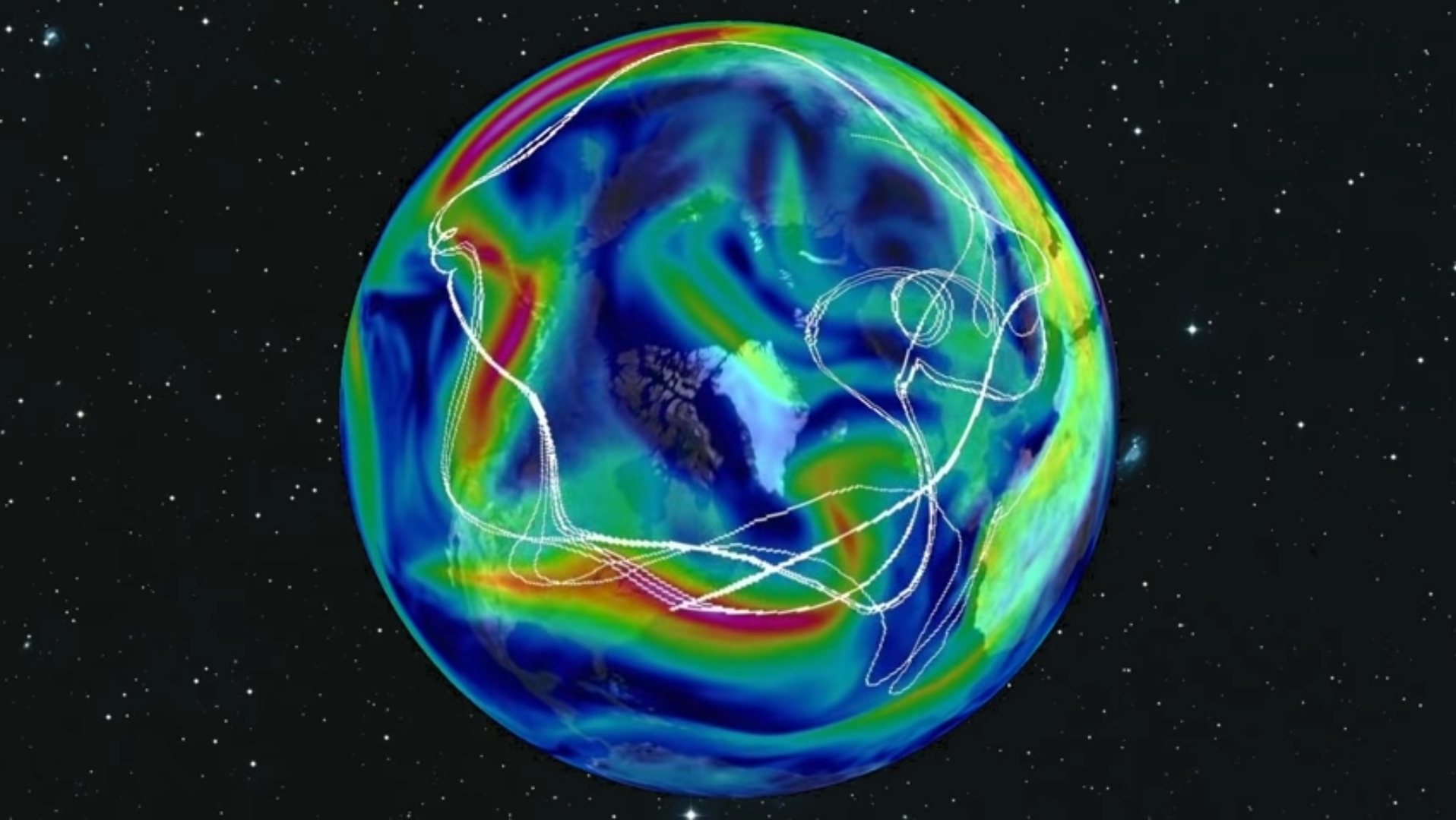The constants \(\sigma\), \(\rho\), and \(\beta\) are system parameters proportional to the Prandtl number, Rayleigh number, and certain physical dimensions of the layer itself where \(\sigma\), \(\rho\), and \(\beta\) are three parameters, with values of\(\sigma = 10,\ \beta= \frac{8}{3}, \rho=28\). Implementation of an IVP ODE in R can be separated into two parts: ‘the model specification’ and the ‘model application’.

The model specification consists of:

• Defining model parameters and their values,

• Defining model state variables and their initial conditions,

• Implementing the model equations that calculate the rate of change (e.g. \(\frac{dx}{dt}\)) of the state variables.

The model application consists of:

• Specification of the time at which model output is wanted,

• Integration of the model equations (uses R-functions from deSolve),

• Plotting of model results.

1.1. MODEL SPECIFICATION

Model parameters:

There are three model parameters: s, r, and b that are defined first. Parameters are stored as a vector with assigned names and values:

parameters <- c(s=10,r=28,b=8/3)

State Variables:

The three state variables are also created as a vector, and their initial values are given:

initial_state <-
  c(x = -8.60632853,
    y = -14.85273055,
    z = 15.53352487)

Model Equation

The model equations are specified in a function (Lorenz) that calculates the rate of change of the state variables. Input to the function is the model time (t, not used here, but required by the calling routine), and the values of the state variables (state) and the parameters, in that order. This function will be called by the R routine that solves the differential equations (here we use ode, see below). The code is most readable if we can address the parameters and state variables by their names. As both parameters and state variables are ‘vectors’, they are converted into a list. The statement with (as. list (c(state, parameters)), …) then makes available the names of this list. The main part of the model calculates the rate of change of the state variables. At the end of the function, these rates of change are returned, packed as a list. Note that it is necessary to return the rate of change in the same ordering as the specification of the state variables. This is very important. In this case, as state variables are specified \(x\) first, then \(y\) and \(z\), the rates of changes are returned as \(dx,dy,dz\).

lorenz <- function(t, state, parameters) {
  with(as.list(c(state, parameters)), {
    dx <- sigma * (y - x)
    dy <- x * (rho - z) - y
    dz <- x * y - beta * z
    
    list(c(dx, dy, dz))
  })
}

1.2. MODEL APPLICATION:

Time Specification

We run the model for 100 days, and give output at 0.01 daily intervals. R’s function seq( ) creates the time sequence:

times <- seq(0, 500, length.out = 125000)

Model Integration

The model is solved using ’deSolve’ function ode, which is the default integration routine. Function ode takes as input, a.o. the state variable vector (y), the times at which output is required (times), the model function that returns the rate of change (func) and the parameter vector (parms). Function ode returns an object of class deSolve with a matrix that contains the values of the state variables (columns) at the requested output times.

lorenz_ts <-
  ode(
    y = initial_state,
    times = times,
    func = lorenz,
    parms = parameters,
    method = "lsoda"
  ) %>% as_tibble()

lorenz_ts[1:10,]

Plotting Results:

Finally, the model output is plotted. We use the plot method designed for objects of class deSolve, which will neatly arrange the figures in two rows and two columns; before plotting, the size of the outer upper margin (the third margin) is increased. We access to \(x\),\(y\),\(z\) respectively a univariate time series. As the time interval used to numerically integrate the differential equations was rather tiny, we just use every tenth observation.

library(deSolve)
library(tidyverse)

parameters <- c(sigma = 10,
                rho = 28,
                beta = 8/3)

initial_state <-
  c(x = -8.60632853,
    y = -14.85273055,
    z = 15.53352487)

lorenz <- function(t, state, parameters) {
  with(as.list(c(state, parameters)), {
    dx <- sigma * (y - x)
    dy <- x * (rho - z) - y
    dz <- x * y - beta * z
    
    list(c(dx, dy, dz))
  })
}

times <- seq(0, 500, length.out = 125000)

lorenz_ts <-
  ode(
    y = initial_state,
    times = times,
    func = lorenz,
    parms = parameters,
    method = "lsoda"
  ) %>% as_tibble()
obs <- lorenz_ts %>%
  select(time, x) %>%
  filter(row_number() %% 10 == 0)
# lorenz_ts[1:10,]

ggplot(obs, aes(time, x)) +
  geom_line() +
  coord_cartesian(xlim = c(0, 100)) +
  theme_classic()

obs <- lorenz_ts %>%
  select(time, y) %>%
  filter(row_number() %% 10 == 0)

ggplot(obs, aes(time, y)) +
  geom_line() +
  coord_cartesian(xlim = c(0, 100)) +
  theme_classic()

obs <- lorenz_ts %>%
  select(time, z) %>%
  filter(row_number() %% 10 == 0)

ggplot(obs, aes(time, z)) +
  geom_line() +
  coord_cartesian(xlim = c(0, 100)) +
  theme_classic()

L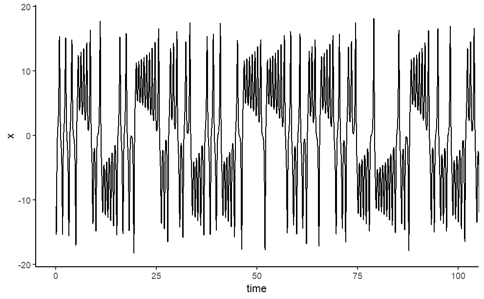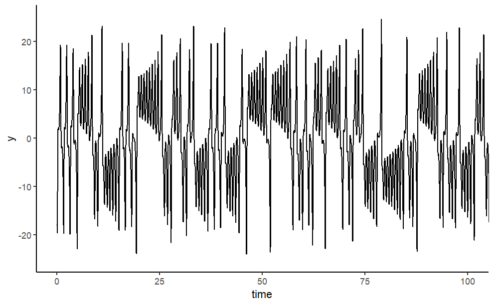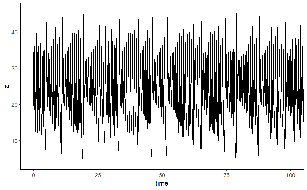orenz Attractor

Let’s try graphing them in three dimensions on a modern computer. The location of the first point is arbitrary. With each point after that, the computer steps forward in time by calculating the position of the next point based on the position of the previous one. It seems to change direction at random, and it never arrives at the same point twice. If it did, that would be the beginning of a repeating pattern. This type of system is now known as a “strange attractor” and this particular one is known as the Lorenz attractor.

library(deSolve)
library(plotly)

parameters <- c(rho = 28, sigma = 10, beta = 8/3)
state <- c(x = 1, y = 1, z = 1)
time <- seq(0, 130, by = 0.01)

lorenz <- function(time, state, parameters) {
  with(as.list(c(state, parameters)), {
    dx <- sigma * (y - x)
    dy <- x * (rho - z) - y
    dz <- x * y - beta * z
    list(c(dx, dy, dz))
  })
}


out <- as.data.frame(ode(y = state, times = time, func = lorenz, parms = parameters))

plot_ly(out, x = ~x, y = ~y, z = ~z, type = 'scatter3d', mode = 'lines', color = ~time, colors = 'Blue')%>% 
  # Set where the camera is set by default
  layout(scene = list(camera = list(eye = list(x = -1, y = 1, z = 0.25))))

Now let’s try drawing 100 points at random locations, and applying the equations to each of them. At first, it will look pretty random but soon a familiar form emerges. The trajectories that began on the edges seem to speed off in random directions. But all those that began within a certain space end up in the attractor. It might seem like their starting positions no longer matter, but once they reach the attractor, their trajectories diverge, each following its path indefinitely, and they never cross. So, the small differences in their start positions lead to increasingly different futures. 

# Package for solving differential equations
library(deSolve)
# Package for interactive 3D plots
library(plotly)
# Specify the equations
lorenz <- function(t, state, parameters) {
  with(as.list(c(state, parameters)), {
    dx <- sigma * (y - x)
    dy <- x * (rho - z) - y
    dz <- x * y - beta * z
    list(c(dx, dy, dz))
  })
}

# Specify parameters
parameters <- c(sigma = 10, beta = 8/3, rho = 28)
# Initial conditions, in the order x, y, z
state <- c(x = 2, y = 3, z = 4)
# Time over which the equations are numerically solved, 25 units
times <- seq(0, 100, 0.01)
# Solve the equations
sol <- as.data.frame(ode(y = state, times = times, func = lorenz, parms = parameters, method = "ode45"))

plot_ly(data = sol, x = ~x, y = ~y, z = ~z) %>%
  add_paths(color = ~time) %>% 
  # Set where the camera is set by default
  layout(scene = list(camera = list(eye = list(x = -1, y = 1, z = 0.25))))

It’s the poster child of chaos theory and is sometimes almost synonymous with the butterfly effect or the field of chaos theory itself. It even looks like a butterfly. A strange attractor is one that has a fractal structure. No point in space is ever visited more than once by the same trajectory. If that happened, the trajectory would travel in a predictable loop and no two trajectories will ever intersect. If that happened, they would merge into the same path, giving two different sets of initial conditions the same outcome i.e., a single trajectory will visit an infinite number of points in this limited space, and this limited space will have an infinite number of trajectories.

library(ggplot2)
library(gganimate)
# Solve differential equations
library(deSolve)
# 3D plots with ggplot2
#library(gg3D)

# Specify the equations
lorenz <- function(t, state, parameters) {
  with(as.list(c(state, parameters)), {
    dx <- sigma * (y - x)
    dy <- x * (rho - z) - y
    dz <- x * y - beta * z
    list(c(dx, dy, dz))
  })
}

# Solve with any initial condition
lorenz_solve <- function(y, t, params) {
  as.data.frame(ode(y = y, times = t, func = lorenz, parms = params, method = "ode45"))
}

# Specify parameters
parameters <- c(sigma = 10, beta = 8/3, rho = 28)
# Time over which the equations are numerically solved, 25 units
times <- seq(0, 25, 0.01)
# Initial conditions, in the order x, y, z
state <- c(x = 2, y = 3, z = 4)
state2 <- c(x = 2, y = 3, z = 4.1)
# Solve
sol <- lorenz_solve(state, times, parameters)
sol2 <- lorenz_solve(state2, times, parameters)
sol$init <- "(2,3,4)"
sol2$init <- "(2,3,4.1)"
# Combine the two solutions into the same data frame for plotting
# I dropped the last time point to get a nice number to get an integer number of frames
sols <- rbind(sol[1:2500,],sol2[1:2500,])

p1 <- ggplot(sols, aes(x, z, color = init)) +
  geom_path(data = sols[,-1], aes(x, z, color = init), size = 0.5) +
  geom_point() +
  scale_color_manual(values = c("#42e5f4", "#f441e2")) +
  # theme with white background
  theme_bw()  +
  # Make sure that units of the axes have the same length
  coord_equal() +
  # Use the time column in the data frame
  transition_time(time = time)
animate(p1, nframes = 2500, fps = 25, renderer = gifski_renderer())

Trajectories are just curves, so they should be 1-dimensional. But how come no matter how much you zoom in on this attractor, you can always find more and more trajectories everywhere?

This is the reason that this attractor is said to have a non-integer dimension. It’s made up of infinitely long curves in a finite space, which are so detailed that they start to partially fill up a higher dimension. It’s not 1 dimensional, 2 dimensional, or 3 dimensional - it’s dimension is somewhere in between. As a result of this non-integer dimension and detail of arbitrarily small scales, the set of points in the Lorenz attractor is a fractal space, and that’s why it’s a strange attractor.

library(deSolve)
library(ggplot2)
parameters <- c(s = 10, b = 8/3)
r <- seq(0, 30, by = 0.05)
state <- c(X = 0, Y = 1, Z = 1)
times <- seq(0, 50, by = 0.01)

Lorenz <- function(t, state, parameters) { 
  with(as.list(c(state, parameters)), {
    dX <- s * (Y - X)
    dY <- X * (r - Z) - Y
    dZ <- X * Y - b * Z
    list(c(dX, dY, dZ))
  })
}
out <- lapply(r,
              function(x){
                ode(y = state,
                    times = times,
                    func = Lorenz,
                    parms = c(r = x, parameters),
                    method = "euler")
              }
)

imageStorePath <- "/attractor-lorenz/" # attach a file path where you will put all the generated images

plots_XZ <- list()
for(i in 1:length(r)) {
  p <- ggplot(data.frame(out[[i]])) + 
    geom_path(aes(x = X, y = Z, colour = Y)) +
    ggtitle(paste0('Lorenz attractor r = ', r[i])) +
    theme(
      axis.text.x = element_blank(),
      axis.title.x = element_blank(),
      axis.text.y = element_blank(),
      axis.title.y = element_blank(),
      axis.ticks = element_blank(),
      panel.background = element_blank(),
      legend.position = "none")
  
   ggsave(filename = paste0(imageStorePath, sprintf('%05.2f', r[i]), '.png'),
          plot = p,
          device = 'png')

  plots_XZ[[i]] <- p
}

library(gifski)
png_files <- list.files("/attractor-lorenz/", pattern = ".*png$", full.names = TRUE)
gifski(png_files, gif_file = "attractor.gif", width = 800, height = 600, delay =0.1)

A strange attractor isn’t necessarily chaotic, but a chaotic attractor will always be strange, and Lorenz attractor is a strange chaotic attractor.

When Lorenz presented his work at a conference in 1963, he ended his talk with an anecdote about a meteorologist who asked whether the flap of a seagull’s wings could change the weather forever. He showed that the appearance of randomness could be well understood within a simple framework of deterministic systems and that it didn’t require excessive complexity at all, it just required one ingredient; the system had to somehow be behaving non-linearly. 

What it means for the system to behave non-linearly i.e., responses aren’t proportional to forces on things. 

Lorenz Deterministic Chaos

Let’s take a look at a simple pendulum. A simple pendulum is a mechanical arrangement that demonstrates periodic motion. This non-linear system is periodic ( it repeats itself over and over again at regular intervals ), meaning it follows a repeating pattern. If we start it twice from approximately the same point, we get approximately the same behavior.

The oscillation of a simple pendulumis a kind of periodic motion bounded between two extreme points. If you analyze the motion of a simple pendulum you will find that the pendulum passes through the mean position only after a definite interval of time. We can also classify the above motion to be oscillatory. An oscillatory is a motion in which the body moves to and fro about a fixed position. So an oscillatory motion can be periodic but it is not necessary.

Graphs are useful because they can take complicated information and display it in a simple, easy-to-read manner. So taking an example of a wave motion we will see some parameters related to periodic motion. Let’s take the following figure:

library(tidyverse)
library(gganimate)
library(gifski)
sine <- data.frame(timer =  seq(from = 0, to =9.9, by = 0.1))
ggplot (sine, aes(x = timer)) + geom_line(aes(y = sin(timer)))
simple_sine <- ggplot (sine, aes(x = timer)) + geom_line(aes(y = sin(timer))) +
  transition_reveal(timer)
animate(simple_sine)

Now let’s try two pendulums connected end to end a non-linear system that’s also non-periodic. If we start it twice from approximately the same position, we will get radically different behavior over time.

library(tidyverse)
library(gganimate)
# constants
G  <-  9.807  # acceleration due to gravity, in m/s^2
L1 <-  1.0    # length of pendulum 1 (m)
L2 <-  1.0    # length of pendulum 2 (m)
M1 <-  1.0    # mass of pendulum 1 (kg)
M2 <-  1.0    # mass of pendulum 2 (kg)

parms <- c(L1,L2,M1,M2,G)

# initial conditions
th1 <-  20.0  # initial angle theta of pendulum 1 (degree)
w1  <-  0.0   # initial angular velocity of pendulum 1 (degrees per second)
th2 <-  180.0 # initial angle theta of pendulum 2 (degree)
w2  <-  0.0   # initial angular velocity of pendulum 2 (degrees per second)

state <- c(th1, w1, th2, w2)*pi/180  #convert degree to radians
derivs <- function(state, t){
  L1 <- parms[1]
  L2 <- parms[2]
  M1 <- parms[3]
  M2 <- parms[4]
  G  <- parms[5]
  
  dydx    <-  rep(0,length(state))
  dydx[1] <-  state[2]
  
  del_ <-  state[3] - state[1]
  den1 <-  (M1 + M2)*L1 - M2*L1*cos(del_)*cos(del_)
  dydx[2]  <-  (M2*L1*state[2]*state[3]*sin(del_)*cos(del_) +
                  M2*G*sin(state[3])*cos(del_) +
                  M2*L2*state[4]*state[4]*sin(del_) -
                  (M1 + M2)*G*sin(state[1]))/den1
  
  dydx[3] <-  state[4]
  
  den2 <-  (L2/L1)*den1
  dydx[4]  <-  (-M2*L2*state[4]*state[4]*sin(del_)*cos(del_) +
                  (M1 + M2)*G*sin(state[1])*cos(del_) -
                  (M1 + M2)*L1*state[2]*state[2]*sin(del_) -
                  (M1 + M2)*G*sin(state[3]))/den2
  
  return(dydx)
}

library(odeintr)
sol <- odeintr::integrate_sys(derivs,init = state,duration = 30,
                              start = 0,step_size = 0.1)

x1 <-  L1*sin(sol[, 2])
y1 <-  -L1*cos(sol[, 2])

x2 <- L2*sin(sol[, 4]) + x1
y2 <- -L2*cos(sol[, 4]) + y1

df <- tibble(t=sol[,1],x1,y1,x2,y2,group=1)


ggplot(df)+
  geom_segment(aes(xend=x1,yend=y1),x=0,y=0)+
  geom_segment(aes(xend=x2,yend=y2,x=x1,y=y1))+
  geom_point(size=5,x=0,y=0)+
  geom_point(aes(x1,y1),col="red",size=M1)+
  geom_point(aes(x2,y2),col="blue",size=M2)+
  scale_y_continuous(limits=c(-2,2))+
  scale_x_continuous(limits=c(-2,2))+
  ggraph::theme_graph()+
  labs(title="{frame_time} s")+
  transition_time(t) -> p

pa <- animate(p,nframes=nrow(df),fps=20)
pa

This is what Lorenz called “Deterministic Chaos”. Deterministic, because its future is determined by physical laws, although it seems random. If the weather works this way, that would explain why it has proven so difficult to predict.

tmp <- select(df,t,x2,y2)
trail <- tibble(x=c(sapply(1:5,function(x) lag(tmp$x2,x))),
                y=c(sapply(1:5,function(x) lag(tmp$y2,x))),
                t=rep(tmp$t,5)) %>% 
  dplyr::filter(!is.na(x))

library(transformr)
ggplot(df)+
  geom_path(data=trail,aes(group=t,x,y),colour="blue",size=0.5)+
  geom_segment(aes(xend=x1,yend=y1),x=0,y=0)+
  geom_segment(aes( xend=x2,yend=y2,x=x1,y=y1))+
  geom_point(size=5,x=0,y=0)+
  geom_point(aes(x1,y1),col="red",size=M1)+
  geom_point(aes(x2,y2),col="blue",size=M2)+
  scale_y_continuous(limits=c(-2,2))+
  scale_x_continuous(limits=c(-2,2))+
  ggraph::theme_graph()+
  labs(title="{frame_time} s")+
  transition_time(t)+
  shadow_mark(colour="grey",size=0.1,exclude_layer = 2:6)-> p_1
pa_1 <- animate(p_1,nframes=nrow(df),fps=20)
pa_1

But what if we could scan our entire planet with extreme precision? As we drastically reduce the errors in our measurements, won’t we eventually be able to predict the weather much further in advance?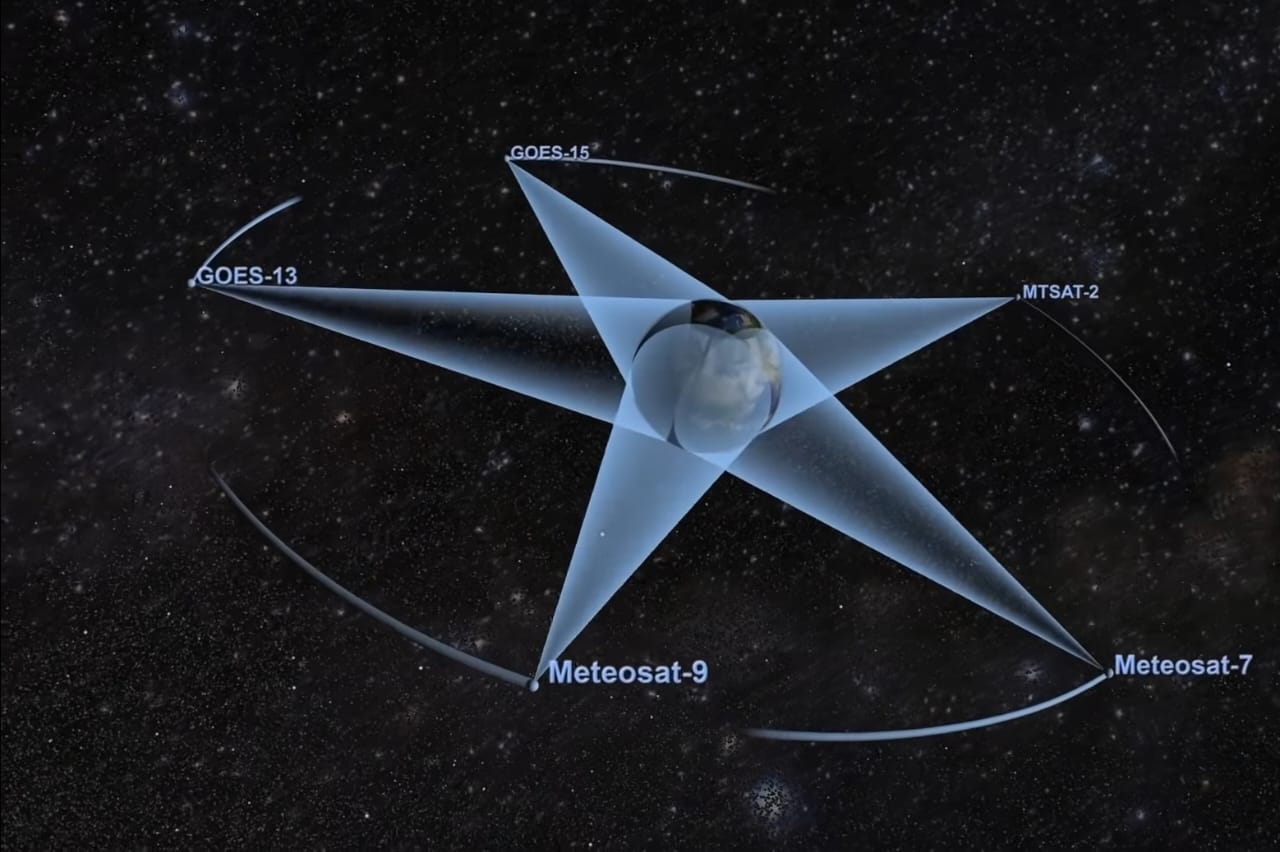

This visualization showcases the five weather satellites that create NOAA’s Climate Prediction Center (CPC) products. The five geosynchronous satellites are: GOES-11, GOES-13, MSG-2, Meteosat-7 and MTSAT-2

Lorenz’s Mathematical Model

In work published in 1969, Lorenz returned to the question of the seagull’s wing by taking a closer look at how tiny motions in the air scale up over time to affect huge systems, and how errors in small-scale measurements evolve into large-scale errors in prediction. He proposed a mathematical model of how this might work and found something surprising: the systems in his model could only be predicted up to a specific point in the future. Beyond that initial error wouldn’t increase the predictability. Lorenz didn’t know for sure that the atmosphere behaves this way, and we still don’t. But this model had major applications because it showed a future determined by physical laws may be no different from one that is completely random, in terms of our ability to predict it beyond a certain point. 

The Butterfly Effect

This was the major challenge to the idea of the Cartesian Universe. The whole idea that certain systems have these finite prediction horizons that you can’t go beyond which was really new. Nobody imagined that to be the case. When Lorenz presented this work at a conference in 1972, the organizer didn’t receive his talk title in time, so he suggested one:

” Does the flap of a butterfly’s wings in Brazil set off a Tornado in Texas?“

So, the butterfly instead of a seagull, became the image most associated with his work. It’s had an increasingly profound impact on a number of disciplines. In its first 10 years, Lorenz’s 1963 paper was cited in about 10 other publications. Since then, it’s been cited over 9,000 times, in papers from nearly every field of science.

In 1987, a popular book by James Gleick introduced the world to the work of Lorenz and other Chaos pioneers, and the ‘Butterfly Effect’ became part of popular culture. 

The butterfly effect is a theory according to which the smallest thing, such as a butterfly flapping its wings can create a series of events leading to a catastrophe, such as a Tornado.

Scientists continue to create mathematical models of more non-linear systems. If those models are correct, deterministic chaos can be found in some fascinating places, including financial markets, as well as the eye movements of people with certain brain disorders; in the onset of sickle-cell disease in the human body; and in the fluctuations of human and animal populations.

In 1992, scientists at MIT used a supercomputer to model our entire solar system almost 100 million years into the future and found it could only be predicted reliably beyond about 12 million years. Beyond that planets could collide with other objects, or be ejected from the system. So, even the motions of the planets, which humans have predicted for centuries, are not quite as simple as we thought. 

Solar system “vortex” gif (by DjSadhu)

The very system we think of as the model of order is unpredictable on even modest timescales. Now a genuine question occurs in our mind i.e., how well can we predict future the future? the answer is, not very well at all at least when it comes to a chaotic system. The further you try to predict the harder it becomes and past a certain point, predictions are no better than guesses. The same is true when looking into the past of chaotic systems and trying to identify initial causes. Intuitively, it is like a fog that sets in the further we try to look into the further or into the past. Chaos puts fundamental limits on what we can know about the future of systems and what we can say about their past. But there is a silver lining.

Let’s look again at the phase space of Lorenz’s equations. If we start with a whole bunch of different initial conditions and watch them evolve, initially the motion is messy. But soon all the points have moved towards or onto an object. The object coincidentally looks a bit like a butterfly. It is the attractor. For a large range of initial conditions, the system evolves into a state on this attractor.

All the paths traced out here never cross and they never connect to from loop, If they did then they would continue on that loop forever and the behavior would be periodic and predictable. So each path here is actually an infinite curve in a finite space.

Lorenz attractor is the most famous example of a chaotic attractor. Though many others have been found for other systems of equations.

If people have heard anything about the butterfly effect, it’s usually about how tiny causes make the future unpredictable, but the science behind the butterfly effect also reveals a deep and beautiful structure underlying the dynamics. One that can provide useful insight into the behavior of a system. So you can’t predict how any individual state will evolve, but you can say how a collection of states evolves and, at least in the case of Lorenz’s equations, they take the shape of a butterfly.

Footnotes

• Strange Attractors: an R experiment about maths, recursivity and creative coding

• Animated graphs in R (and a little about bifurcation, chaos and attractors).

See Also

• Bifurcation and Beginning of Chaos

• Unveiling the Feigenbaum Ballet of Sine Dynamics

• Beauty in the Midst of Chaos

References

1. “chaos theory | Definition & Facts”. Encyclopedia Britannica. Retrieved 2019-11-24.

2. Keydana (2020, June 24). Posit AI Blog: Deep attractors: Where deep learning meets chaos.

3. Chaos: Making a New Science by James Gleick.

4. Gilpin, William. 2020. “Deep Reconstruction of Strange Attractors from Time Series.”

5. Strang, Gilbert. 2019. Linear Algebra and Learning from Data. Wellesley Cambridge Press.

6. Strogatz, Steven. 2015. Nonlinear Dynamics and Chaos: With Applications to Physics, Biology, Chemistry, and Engineering. Westview Press.