Integration of Inverse Functions
God does not care about our mathematical difficulties. He integrates empirically.— Albert Einstein
\(\text{Inverse Integral Set-up}\)
\(\text{Integration of inverse functions can be computed by means of a formula that expresses}\) \(\text{the}\) \(\text{indefinite integral of the inverse}\) \(f^{-1}\) \(\text{of a continuous and}\) invertible function \(f\), \(\text{in terms of}\) \(f^{-1}\) \(\text{and}\) \(\text{an indefinite integration of}\) \(f\).
\(\text{Statement of The Theorem}\)
\(\text{Suppose},\) \(\text{I}_1\; \text{and} \; \text{I}_2\) \(\text{be two intervals of}\) \(\mathbb{R}\). \(\text{Assuming that}\) \(f: I_1 \rightarrow I_2\) \(\text{is a continuous}\) \(\text{and invertible function. It follows from the}\) intermediate value theorem \(\text{that}\) \(f\) \(\text{is strictly monotone. Since}\) \(f\) \(\text{and the inverse function}\) \(f^{-1}: I_2 \rightarrow I_1\) \(\text{are continuous,}\) \(\text{they}\) \(\text{have}\) \(\text{indefinite integration by the}\) fundamental theorem of calculus.
\(\int f^{-1}(y)dy\;\; \text {is the typical notation of inverse integral. We will solve this integral using integration}\) \(\text{by parts. Also, we have to use substitution.}\)
\(\text{So, We have,}\) \[I=\int f^{-1}(y)dy\] \(\text{Let us assume,}\ x = f^{-1}(y)\; \text{where}\; y=f(x)\) \(\therefore\; y=f(x)\implies dy = d(f(x))=df(x)\)
\(\text{Here we will write our integrand in terms of} \; x\). \(\text{Therefore,}\)
\[ I=\int f^{-1}(f(x))\ df(x)= \int x\ df(x) \]
\(\text{Here, we will apply the integration by parts to solve the above integral.}\)\[\int x\ df(x)= x\int df(x)\ - \int \bigg[\dfrac{d}{dx}(x) \int df(x)\bigg]dx\]
\[= xf(x)\ - \int f(x)dx\]
\[ =xf(x)-F(x)+C \]
\[ \;\;= yf^{-1}(y)-F(f^{-1}(y))+ C \]
\[ \therefore \boxed{\ \int f^{-1}(y)dy = yf^{-1}(y)\ - F \circ f^{-1}(y)+C} \hspace{0.8 cm} \ldots (*) \]
\(\text{Problem 1}\)
\(\text{Approch 1 :}\)
\(\text{If}\) \(f\) \(\text{be a decreasing and continuous function on}\) \([a,b]\), \(\text{then prove that}\)
\[ \int_{f(b)}^{f(a)} f^{-1}(y)dy\ = af(a)-bf(b)+\int_a^b f(x)dx \]
\(\text{We shall express}\) \(\int_{f(b)}^{f(a)} f^{-1}(y)dy\) \(\text{ in terms of }\) \(x\) \(\text{ instead of}\) \(y\).
\[ \int_{f(b)}^{f(a)} f^{-1}(x)dx \]
\(\text{Using the fact that},\) \[\int f^{-1}(y)dy =yf^{-1}(y)-F(f^{-1}(y))+ C\]
\(\text{where}\) \(F\) \(\text{is the indefinite integral of}\) \(f\), \(\text{we can obtain},\)
\[ \int_{f(b)}^{f(a)} f^{-1}(x)dx = \left[{xf^{-1}(x) - F(f^{-1}(x))}\right]^{f(a)}_{f(b)} \]
\[ \hspace{2.7 cm}= f(a)a - F(a) - (f(b)b - F(b)) \]
\[ \boxed{\int^{f(b)}_{f(a)} f^{-1}(x)dx = F(a) - F(b) - af(a)+bf(b)} \]
\(\text{Now},\)
\[ \int_a^b f(x)dx + \int^{f(b)}_{f(a)} f^{-1}(x)dx \]
\[ = F(b) - F(a) + F(a) - F(b) - af(a)+bf(b) \]
\[ \therefore \int_a^b f(x)dx + \int^{f(b)}_{f(a)} f^{-1}(x)dx = - af(a)+bf(b) \]
\[ \implies -\int^{f(b)}_{f(a)} f^{-1}(x)dx = af(a)-bf(b) + \int_a^b f(x)dx \]
\[ \implies \boxed{\int^{f(a)}_{f(b)} f^{-1}(x)dx = af(a)-bf(b) + \int_a^b f(x)dx} \] \(\text{Hence, we are done.}\)
\(\text{We can also do this problem by integration by parts. For the convention of reder, it is shown below.}\)
\(\text{Approach 2:}\)
\(\text{Let's define}\) \(f^{-1}(y)=t \Leftrightarrow y=f(t) \Leftrightarrow dy=f'(t)dt\) \(\text{then we get},\)
\[ \int_{f(b)}^{f(a)} f^{-1}(y)dy=\int_{b}^{a} tf^{'}(t)dt \]
\(\text{Then using integration by parts we get},\)
\[ \int_{b}^{a} tf^{'}(t)dt=tf(t)|_{b}^{a} -\int_{b}^{a}f(t)dt=af(a)-bf(b)-\int_{b}^{a}f(x)dx\]
\(\text{Changing variable t to x we get that,}\)
\[ \int_{f(b)}^{f(a)} f^{-1}(y)dy -\int_a^b f(x)dx=af(a)-bf(b)-\int_{b}^{a}f(x)dx-\int_a^b f(x)dx=af(a)-bf(b) \]
\[ \implies \boxed{\int_{f(b)}^{f(a)} f^{-1}(y)dy = af(a)-bf(b)+\int_a^b f(x)dx} \]
\(\text{Problem 2}\)
\(f:[0,1] \rightarrow [0,1]\) \(\text{is continuous f(0)=0,f(1)=1}\). \(\int_0^1 f(x)dx=\frac{1}{3}\) \(\text{and f is invertible. Find the value of}\)
\[ \int_0^1 f^{-1}(y)dy \]
\(\text{There are two ways of doing this problem. Let us explore the geometrical method first.}\) \(\text{This method}\) \(\text{will provide you a visual understanding.}\)
\(\text{We know that f(0) = 0, f(1) = 1 and f is invertible which means it always passes the horizontal line}\) \(\text{test.}\)
\(\text{Note that,}\) \(\text{An invertible function}\) \(f:[0,0]\rightarrow[1,1]\) \(\text{is either strictly increasing or strictly decreasing.}\) \(\text{So, in this case, it is strictly increasing. Because if it is not strictly increasing then at some point,}\) \(\text{it goes up and it goes down and in that case it would not pass the horizontal line test. That's why in}\) \(\text{this case, it's strictly increasing. Moreover, we know that }\) \(\int_0^1 f(x)dx = \frac{1}{3}\)
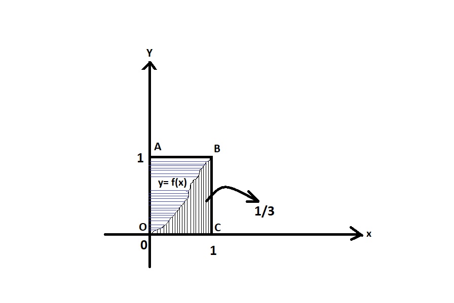
\(\therefore\) \(\text{OBC} = \dfrac{1}{3} .\) \(\text{As the curve OB i.e., the function}\) \(y=f(x)\) \(\text{is invertible then we can solve for}\) \(x\) \(\text{and we get}\) \(x=f^{-1}(y).\) \(\text{But our objective is to figure out}\) \(\int_0^{1} f^{-1}(y)dy.\)
\(\text{If you tilt your head and the interesting thing is this is not the graph of}\; f\; \text{but in terms of}\; y\;\) \(\text{this is the graph of}\; f^{-1}(y).\) \(\text{Notice that area of OAB is precisely}\) \(\text{ABCO}-\text{OBC}.\)
\(\therefore \text{Our answer would be ( area of the ABCO} - \text{area of OBC)} =(1-\frac{1}{3}) = \frac{2}{3}.\)
\(\text{Another solution of this problem can be written as,}\)
\[ \int_0^1 f^{-1}(y)dy \]
\(\text{Let us substitute}\; y=f(x) \implies dy=f^{'}(x)dx.\) \(\text{Notice that,}\) \(f(0)=0=f(x) \implies x = 0.\) \(\text{Similarly,}\; f(1)=1=f(x)\implies x=1.\) \(\text{Therefore we can substitute above integral as,}\)
\[ \int_0^1 f^{-1}(y) dy = \big[xf(x)\big]_0^1 \ - \int_0^1 f(x)dx \]
\[ \hspace{4 cm} = f(1)-\int_0^1 f(x)dx = 1- \dfrac{1}{3} = \dfrac{2}{3} \]
\[ \therefore \boxed{\int_0^1f^{-1}(y)dy = \dfrac{2}{3}} \]
\(\text{Problem 3}\)
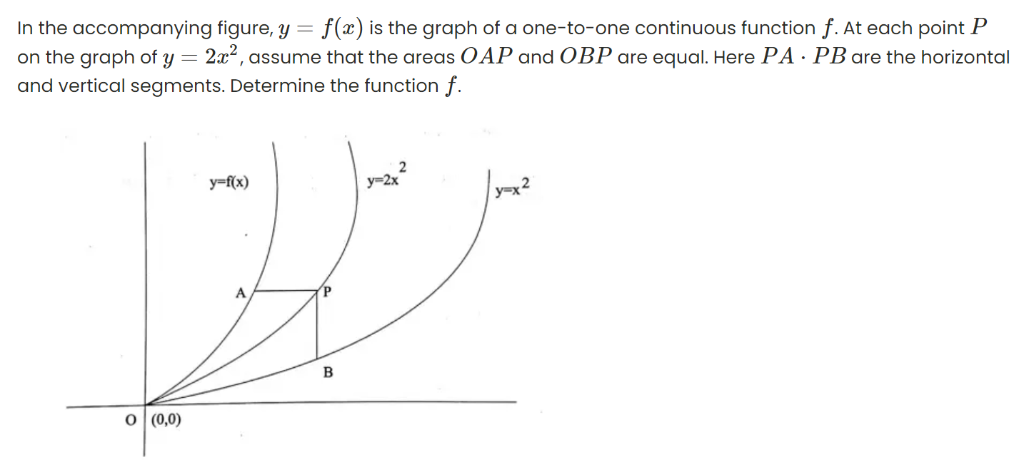
\(\text{Let us assume A}\) \((x_0,y_0),\) \(\text{B}\bigg(\sqrt{\frac{y_0}{2}},\frac{y_0}{2}\bigg)\) \(\text{P}\bigg(\sqrt{\frac{y_0}{2}},y_0\bigg).\) \(\text{Moreover it's given that}\) \(y=2x^2\; \text{or}, x=\sqrt{\frac{y}{2}}.\) \(\text{The area(OPB),}\)
\[ \int_0^{\sqrt{\frac{y_0}{2}}} (2x^2-x^2)dx =\int_0^{\sqrt{\frac{y_0}{2}}} x^2dx \]
\[ \hspace{3 cm}=\bigg[\dfrac{1}{3}x^3\bigg]_0^{\sqrt{\frac{y_0}{2}}} \]
\[ \hspace{2.5 cm}= \dfrac{y_0^{\frac{3}{2}}}{6\sqrt{2}} \] \(\text{The area of OPA will be figuring out with respect to y-axis.}\) \(\text{The area (OPA)},\)
\[ \int_0^{y_0}\bigg(\sqrt{\dfrac{y}{2}}\ - f^{-1}(y)\bigg)dy \]
\[ = \int_0^{y_0}\sqrt{\dfrac{y}{2}}dy\ - \int_0^{y_0}f^{-1}(y)dy \]
\[ = \frac{2}{3\sqrt{2}} y_0^{\frac{3}{2}}-\int_0^{y_0}f^{-1}(y)dy \]
\(\text{As, the areas of OAP and OBP are equal. Therefore, }\)
\[ \frac{2}{3\sqrt{2}} y_0^{\frac{3}{2}}-\int_0^{y_0}f^{-1}(y)dy = \dfrac{y_0^{\frac{3}{2}}}{6\sqrt{2}} \]
\(\text{Differentiate both side with respect to}\;y_0\;\)
\[ \implies \sqrt{\dfrac{y_0}{2}}-f^{-1}(y_0)=\dfrac{1}{4}\sqrt{\dfrac{y_0}{2}} \]
\[ \implies f^{-1}(y_0) = \dfrac{3}{4}\sqrt{\dfrac{y_0}{2}} \]
\[ \therefore y_0 = f \bigg(\dfrac{3}{4}\sqrt{\dfrac{y_0}{2}}\bigg) \]
\(\text{Let us assume}\; \dfrac{3}{4}\sqrt{\dfrac{y_0}{2}} = x \implies y_0 = \frac{32 x^2}{9} , \text{hence}\; \boxed{f(x) = \frac{32x^2}{9}}\)
\(\text{See Also}\)
\(\text{References}\)
Key, E. (Mar 1994). “Disks, Shells, and Integrals of Inverse Functions”. The College Mathematics Journal. 25 (2): 136–138.
Bensimhoun, Michael (2013). “On the antiderivative of inverse functions”. arXiv:1312.3839 [math.HO].
Parker, F. D. (Jun–Jul 1955). “Integrals of inverse functions”. The American Mathematical Monthly. 62 (6): 439–440. doi:10.2307/2307006. JSTOR 2307006.