Dynamics of Julia Sets in Rational Maps
Control and Synchronization with Complex Perturbations
Control Map & Optimal Control Function
- Definition
- The Base System and Rational Map:
- Introducing the Nonlinear Control:
- Fixed Points and Behavior:
- Escape Criterion:
- Generalized Map:
- Visualization Algorithm: Escape-Time Algorithm
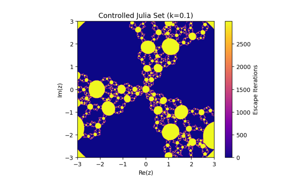
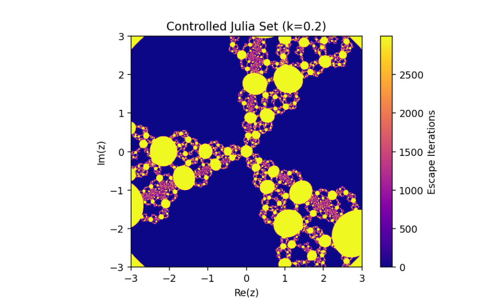
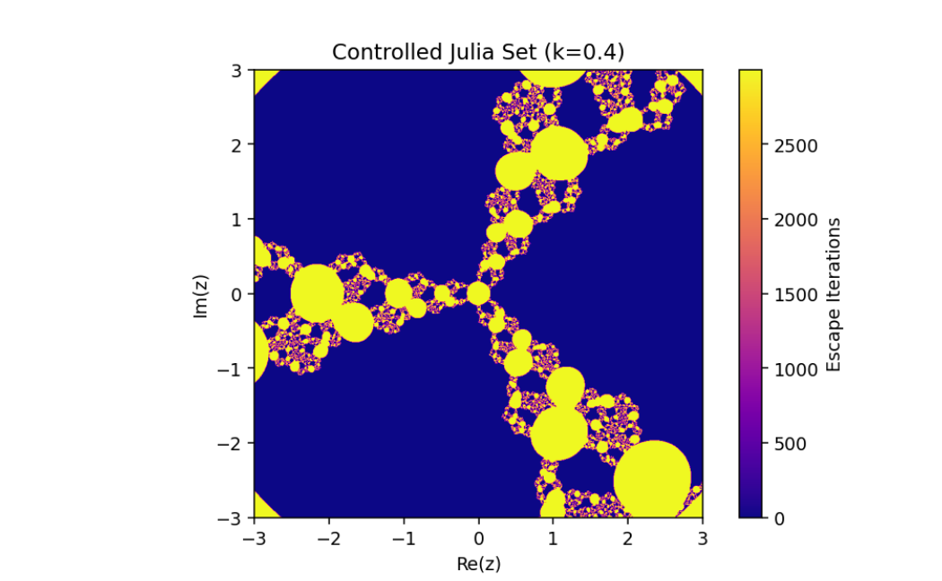
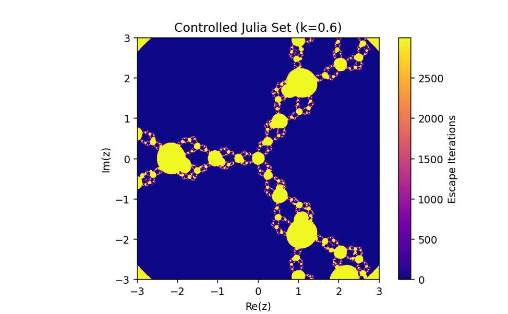
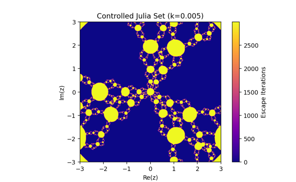
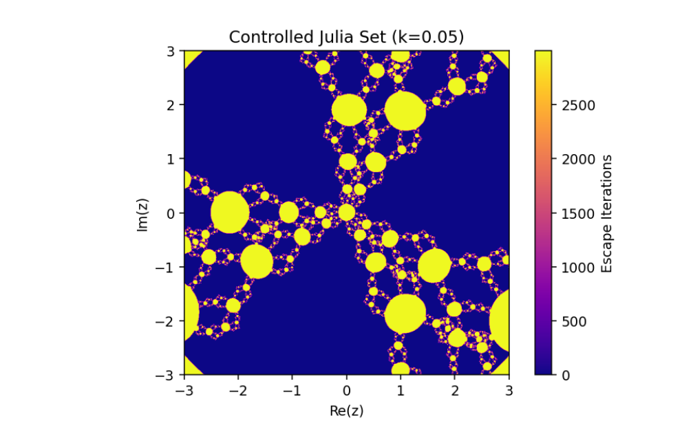
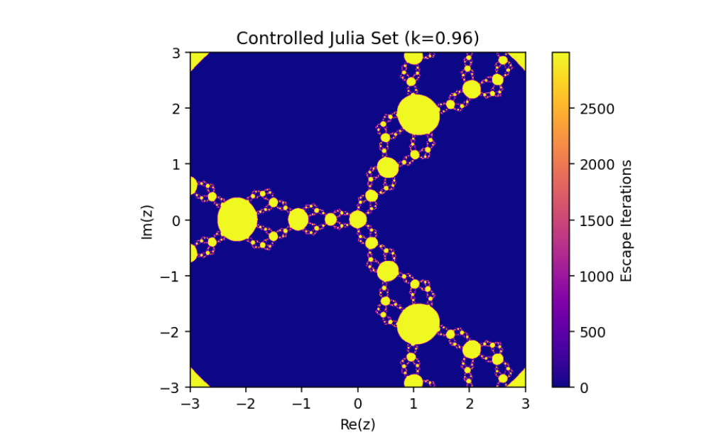
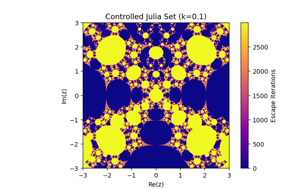
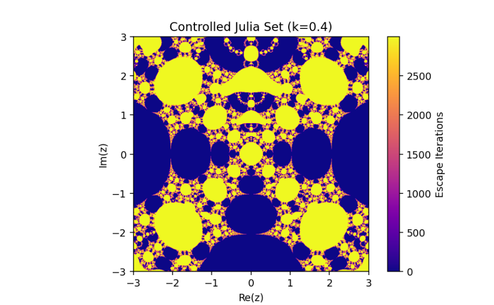
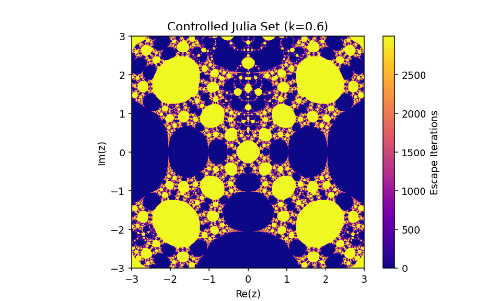
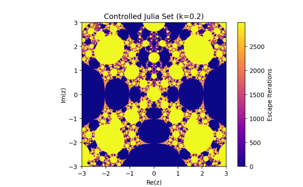
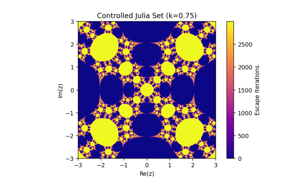
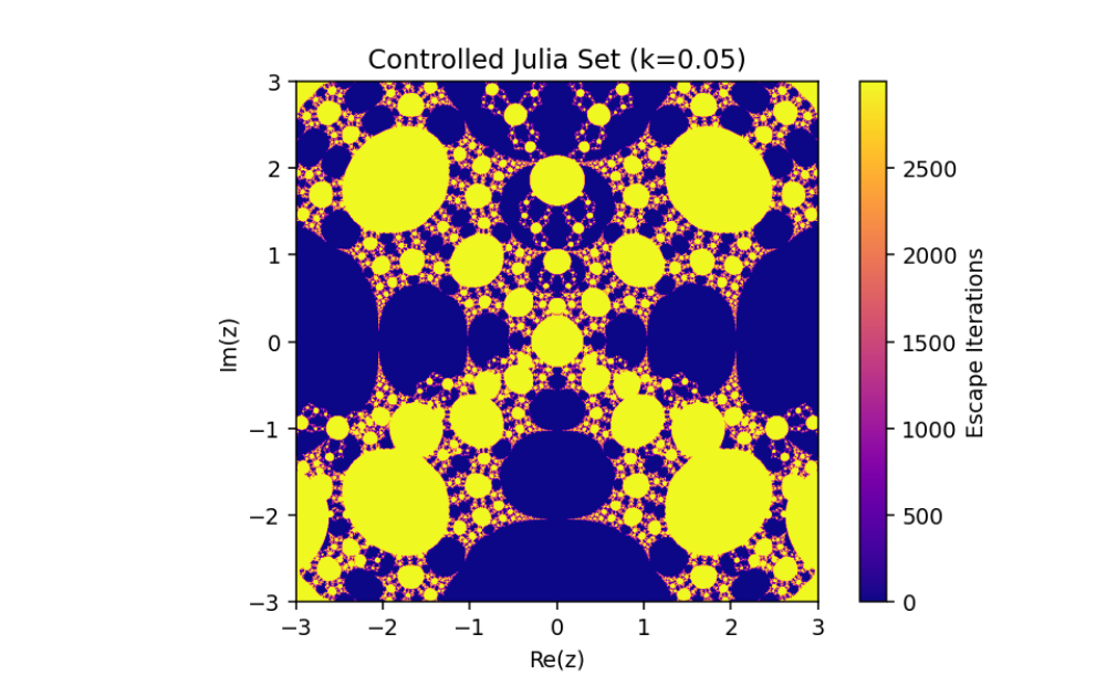
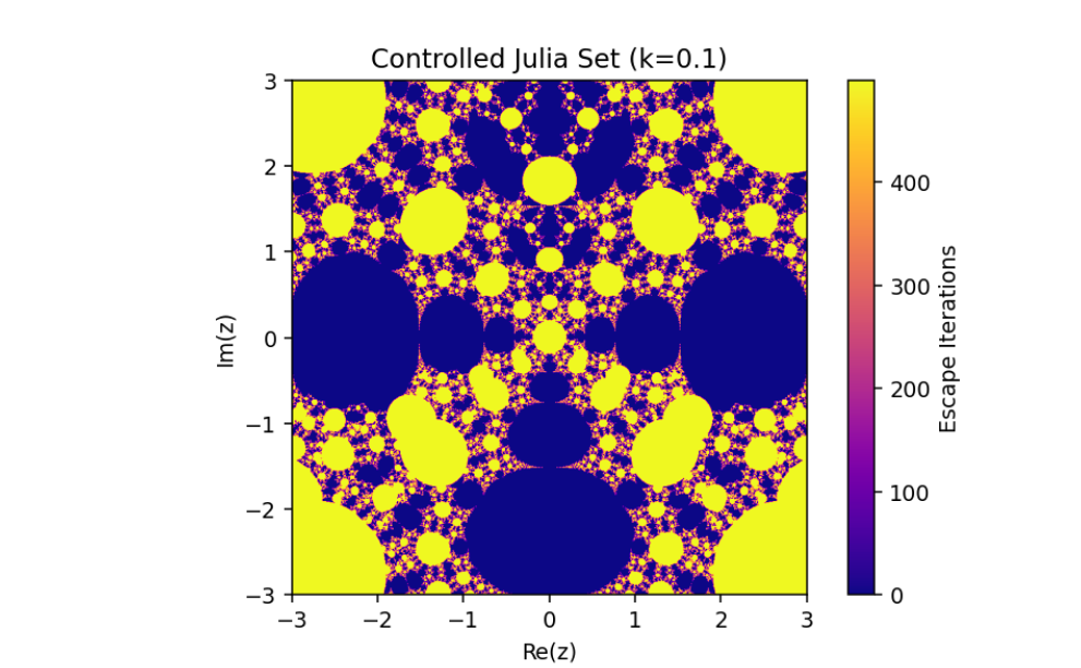
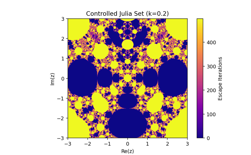
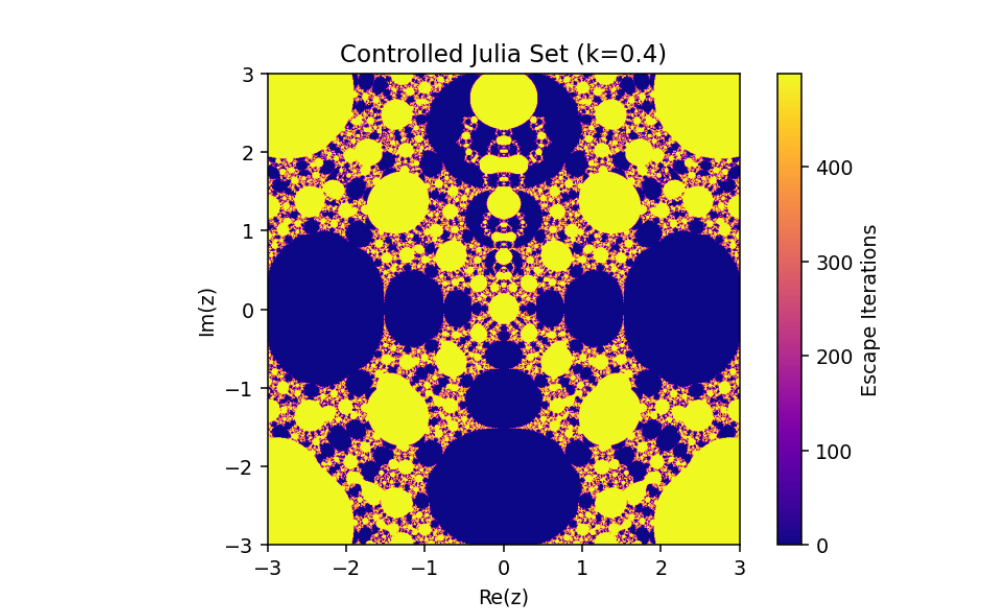
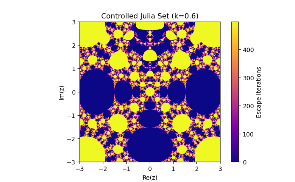
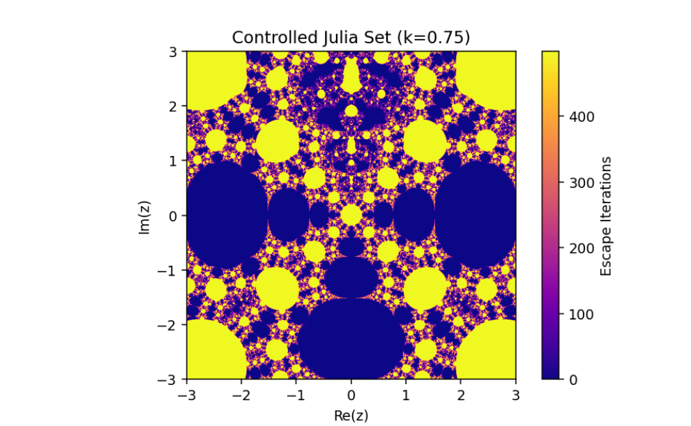
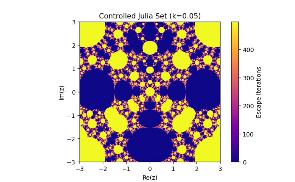
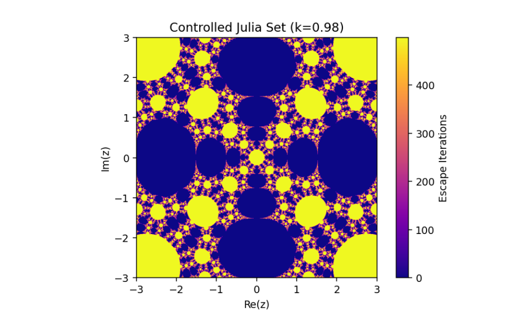
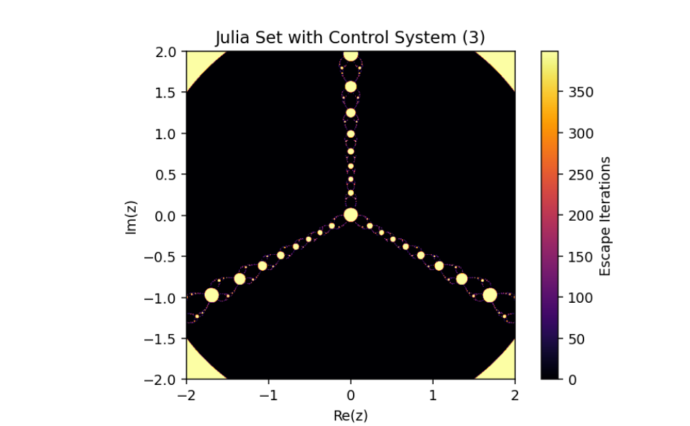
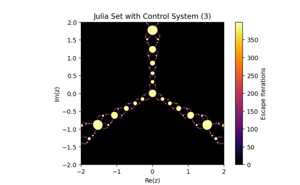
A control parameter \(k\) is introduced to modify the dynamics of the map. The controlled map is defined as:
\[ g(z) = f(z) - k \cdot (f(z) - z) \]
Interpretation:
Base Map Contribution: The term \(f(z)\) represents the original rational Julia map.
Feedback Control: The term \(k \cdot (f(z) - z)\) acts as a damping factor. The control parameter \(k\) (with \(0 \leq k \leq 1\)) adjusts the extent to which the new value depends on the previous iteration.
When \(k=0\), \(g(z) = f(z)\), recovering the original Julia map. When \(k=1\), the map becomes stationary.
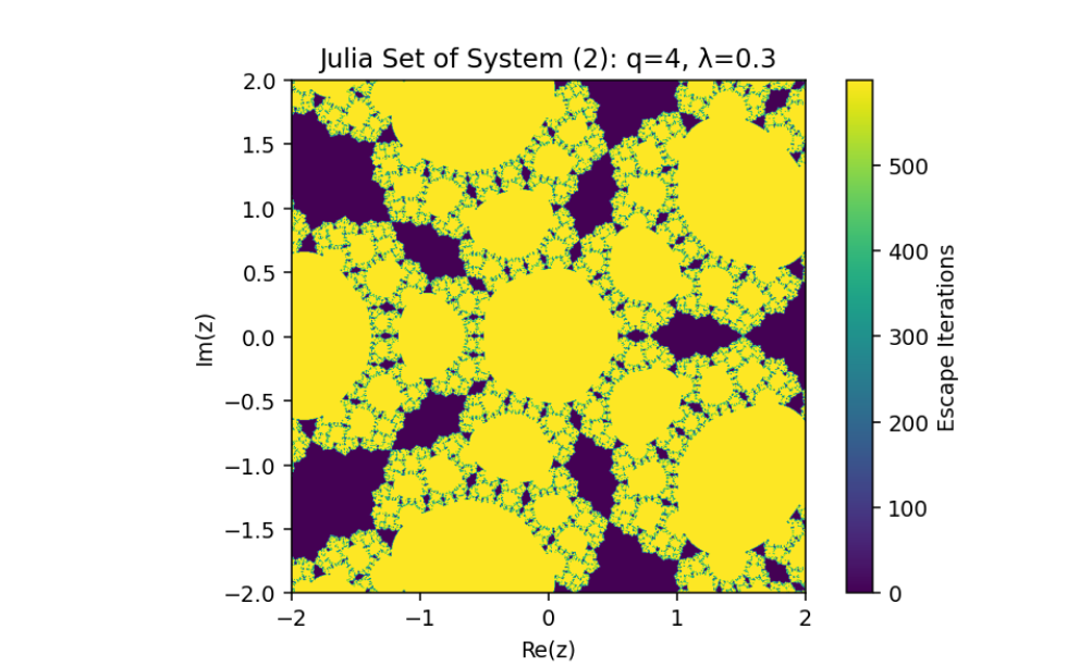
The base system is:
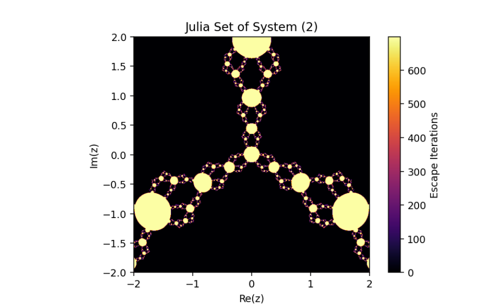
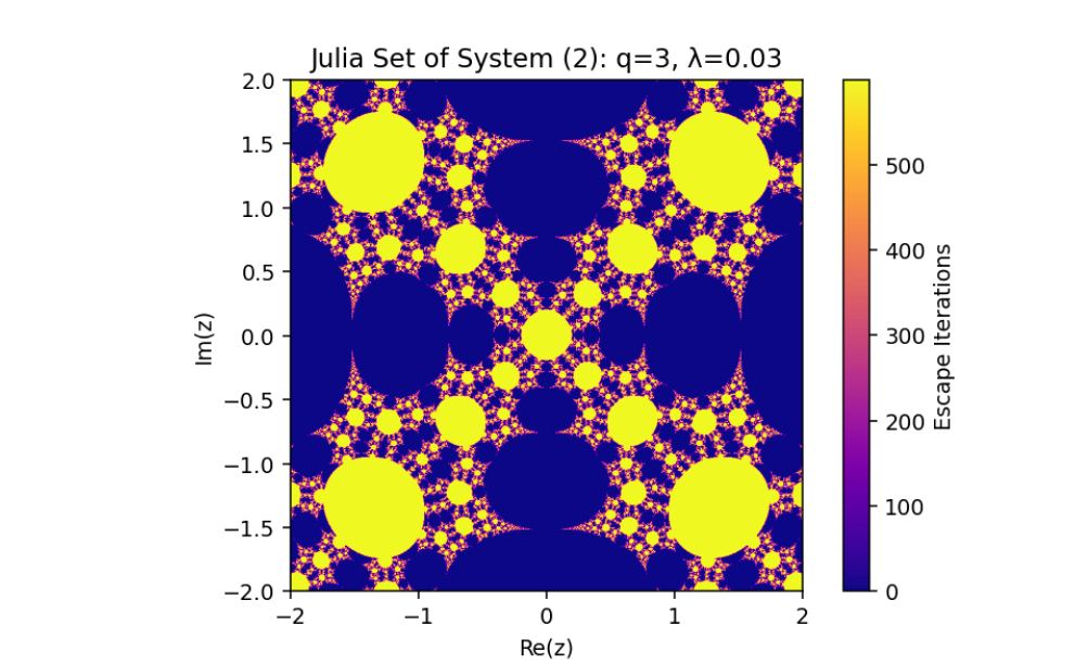
\[ z_{n+1} = f_{\lambda, q}(z_n) = \frac{1}{2} \left(z_n + \frac{\lambda}{z_n^q}\right) \hspace{1 cm} ...(2) \]
which can also be written as:
\[f_{\lambda, q}(z) = \frac{z^{q+1} + \lambda}{2z^q}.\]
This is a rational map where:
The numerator \(P(z) = z^{q+1} + \lambda\),
The denominator \(Q(z) = 2z^q\).
To control the dynamics, a nonlinear control term \(u_n\) is introduced:
\[ u_n = -k[f_{\lambda, q}(z_n) - z_n]. \]
The controlled system becomes:
\[ z_{n+1} = f_{\lambda, q}(z_n) + u_n \]
or equivalently:
\[ z_{n+1} = f_{\lambda, q}(z_n) - k[f_{\lambda, q}(z_n) - z_n] \]
Substitute \(f_{\lambda, q}(z_n) = \frac{1}{2} \left(z_n + \frac{\lambda}{z_n^q}\right)\) into the controlled system:
\[ z_{n+1} = \frac{1}{2} \cdot \left(z_n + \frac{\lambda}{z_n^q}\right) - k \cdot \left[\frac{1}{2} \cdot \left(z_n + \frac{\lambda}{z_n^q}\right) - z_n\right] \hspace{1.5 cm} ...(3) \]
This is a concise symbolic representation called controlled rational map, and we define this following way:
\[\boxed{ R(z)=\frac{(1+k) z_n^{q+1} + \lambda (1-k)}{2 z_n^q}}\]
Fixed Points: The fixed points are solutions of \(R(z)=z\), which reduce to solving:
\[ \frac{(1+k) z^{q+1} + (1-k)\lambda}{2z^q} = z \]
Rearrange:
\[ (1+k) z^{q+1} + (1-k)\lambda = 2z^{q+1} \]
Factorize:
\[ (1+k - 2)z^{q+1} = -(1-k)\lambda \]
Attracting Fixed Point: If \(∣1+k∣>2\), infinity becomes an attracting fixed point.
That’s how we can write:
\[ |R(z)| > |z| \quad \text{for} \quad |z| > M \]
where \(M\) is a threshold beyond which iterates escape to infinity. Using bounds, the escape criterion simplifies to:
\[ |R(z)| = \left|\frac{(1+k) z^{q+1} + (1-k)\lambda}{2z^q}\right| > |z| \]
The control parameter \(k\) influences the structure of the Julia set.
As \(∣1+k∣>2\), infinity becomes an attracting fixed point, shrinking the Julia set.
The escape criterion ensures iterates either escape to infinity or remain bounded within the Julia set boundary.
Iterative Function:
\[z_{n+1} = z_n^q + c + \frac{\lambda}{z_n^p}\]where:
\(p,q \in \mathbb{Z}^+\), are positive integers.
\(\lambda, c \in \mathbb{C}\) are complex parameters.
\(z_n \in \mathbb{C}\) is the iterated sequence.
Boundedness Criterion:
A point \(z_0\) in the complex plane belongs to the filled Julia set if its orbit \(\{z_0, z_1, z_2, \dots\}\) remains bounded under iteration.
For practical purposes, we compute boundedness using an escape radius \(R\):
If \(|z_n| > R\), the point escapes to infinity.
Otherwise, it is bounded.
Key Parameters:
\(q\): Controls the growth of the polynomial term.
\(\lambda\): Perturbation parameter that introduces singularities at the origin.
\(p\): Governs the strength of the singularity.
\(c\): Determines the central point of the hyperbolic component in the Mandelbrot set.
Steps:
Initialize Grid:
- Define a grid of points in the complex plane \(z_0\), e.g., \(x, y \in [-2, 2]\).
Iterative Mapping:
For each \(z_0\), compute its orbit:
\[ z_{n+1} = z_n^q + c + \frac{\lambda}{z_n^p} \]
Escape-Time Calculation:
Track the number of iterations \(n\) required for \(|z_n|\) to exceed a given escape radius \(R\).
Assign a colour to \(z_0\) based on \(n\) (e.g., gradient or palette).
Edge Cases:
Points where \(z_n\) diverges rapidly (\(|z_n| \to \infty\)) are coloured differently.
Points that remain bounded ( \(|z_n| \leq R\) after the maximum iteration) are typically coloured black (belong to the Julia set).
A Descriptive Approach Synchronization of Julia Sets
- Mathematical Settings
- Mathematical Interpretation
- Controlled System (5) when \(q=2,p=2, \lambda =0.073i\)
- Controlled System (5) when \(q=2,p=3, \lambda =0.073i,\mu =0.1\)
- Controlled System (5) when \(q=2,p=3, \lambda =0.073i,\mu=0.03\)
This phenomenon arises in the study of coupled systems, particularly in complex dynamics, where multiple Julia sets, associated with different parameters, exhibit coordinated behavior. Synchronization involves aligning the trajectories and fractal properties of two systems:
Driving System:
\[w_{n+1} = \frac{1}{2} \left( w_n + \frac{\mu}{w_n^p} \right) \text{with parameters}\; p, \mu. \hspace{1 cm} ...(4)\]
Response System:
\[z_{n+1} = R(z_n) - k[R(z_n) - R(w_n)]\]
Synchronization is achieved when the trajectory difference: \(|z_{n+1} - w_{n+1}| \to 0, \text{as}\; k \to 1.\)
Why Synchronization Works
Synchronization is feasible because:
Both systems originate from the same functional framework.
Differences are limited to parameter variations (\(\lambda\) , \(q\)).
The coupling mechanism effectively bridges the gap created by these parameter differences, aligning the trajectories and fractal properties.
The equation provided is:
\[ z_{n+1} = \frac{1}{2} \left( z_n + \frac{\lambda}{z_n^q} \right) - k \left[ \frac{1}{2} \left( z_n + \frac{\lambda}{z_n^q} \right) - \frac{1}{2} \left( w_n + \frac{\mu}{w_n^p} \right) \right] \hspace{1 cm} ...(5) \]
where:
\(z_n\): Represents the primary iterated complex variable.
\(w_n\): Represents a secondary complex variable interacting with \(z_n\).
\(\lambda\): A complex parameter controlling the rational map dynamics.
\(\mu\): Another complex parameter that modifies the \(w_n\) dependent term.
\(p,q\): Positive integers controlling the degree of the respective rational maps.
\(k\): A feedback control parameter.
a modified version of a Julia set generated by introducing a control mechanism into the dynamics of a rational map.
This mechanism alters the behavior of the system, enabling adjustments to its fractal properties based on a coupling or control parameter \(k\). Let’s break down this system and analyze its mathematical structure:
Base Map Contribution:
\[ \frac{1}{2} \left( z_n + \frac{\lambda}{z_n^q} \right) \]
forms the unperturbed Julia set, as seen in System (2).
Secondary Influence:
\[ \frac{1}{2} \left( w_n + \frac{\mu}{w_n^p} \right) \]
introduces a coupling between the \(z_n\) and \(w_n\) dynamics, with the parameter \(\mu\) adjusting this interaction.
Control Mechanism: The term:
\[ - k \left[ \frac{1}{2} \left( z_n + \frac{\lambda}{z_n^q} \right) - \frac{1}{2} \left( w_n + \frac{\mu}{w_n^p} \right) \right] \]
applies feedback that synchronizes the \(z_n\) and \(w_n\) based maps, creating a controlled fractal structure. The control parameter \(k\) determines the extent of this feedback.
This system describes a coupled rational map with feedback control, where:
Coupling: The term involving \(w_n\) and \(\mu/w_n^p\) introduces a synchronized perturbation to the primary Julia set, ensuring dynamic interactions between \(z_n\) and \(w_n\).
Feedback: The parameter \(k\) acts as a regulator, controlling the influence of the coupling term and modifying the convergence or divergence of points in the fractal.