Investigation of the Intricate Universe of Fractals
Origins in Dynamical Systems
- Complex dynamics stemmed from early 20th-century studies by Henri Poincaré.
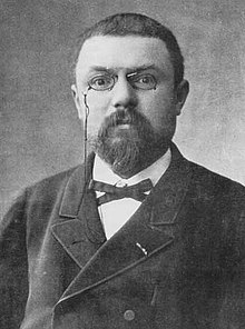
- Foundation for Chaos Theory was laid through the study of dynamical systems.
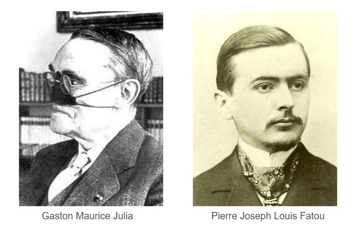
Contributions of Fatou and Julia:
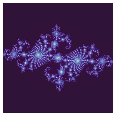
Pierre Fatou and Gaston Julia independently explored the iteration of functions in the complex plane.
![]()
Introduced the concepts of Julia sets and Fatou sets to describe regions of stability and chaos in dynamical systems.
Focused on understanding stability and chaotic behavior through iterations.
Mandelbrot’s Role
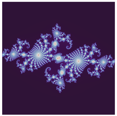
In the 1970s, Benoit Mandelbrot popularized fractals, bringing attention to the work of Fatou and Julia.
![]()
Introduced fractal geometry, highlighting the self-similar and infinitely complex structures from iterative processes.
Mandelbrot set became a visual and mathematical example of fractal geometry.

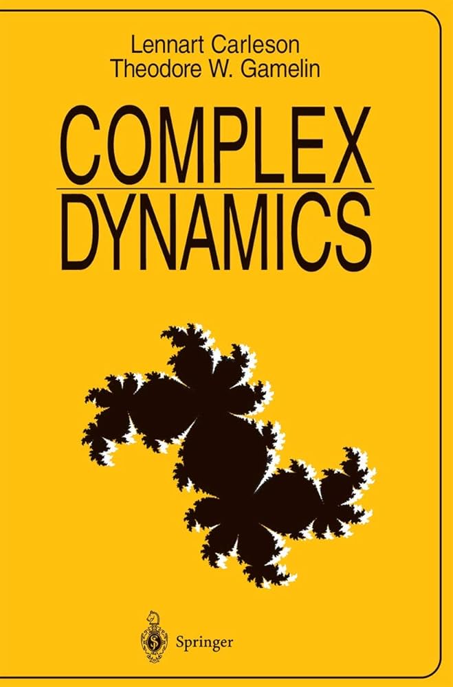
Books & Foundation

Iterations & the Julia Set
The Julia set of a complex function \(f(z)\) is the closure of the set of repelling periodic points of \(f.\) Formally, it is defined as:
\[ J(f) = \{ z \in \mathbb{C} \ | \ \text{the behavior of } f^n(z) \text{ is highly sensitive to initial conditions} \}. \]
The Julia set \(J(f)\) is the boundary of the set of points that remain bounded under iteration of \(f\). It is the set of points where the iterates of \(f\) exhibit chaotic behavior, meaning that small perturbations in the initial conditions result in drastically different long-term outcomes.
The Julia set \(J(f)\) is closed and non-empty.
If \(f\) is a rational map of degree \(d \geq 2\), then \(J(f)\) is a perfect set, meaning it is closed and has no isolated points.
The Julia set is the set of points where the function’s behavior is neither stable nor periodic, often leading to fractal structures.
Interactive Visualization
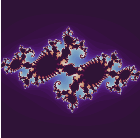
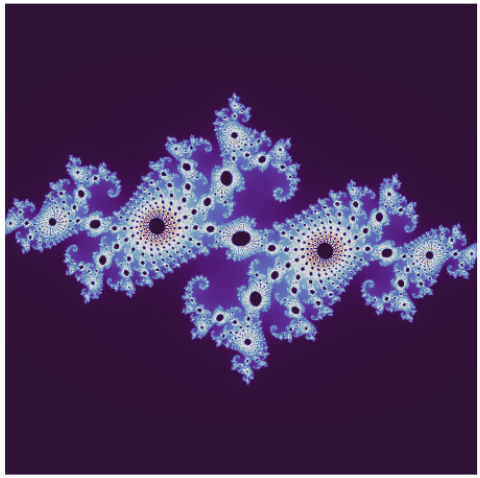
Filled In Julia Set
- Introduction
- Types of Orbits
- Filled Julia Set / Basin of Infinity
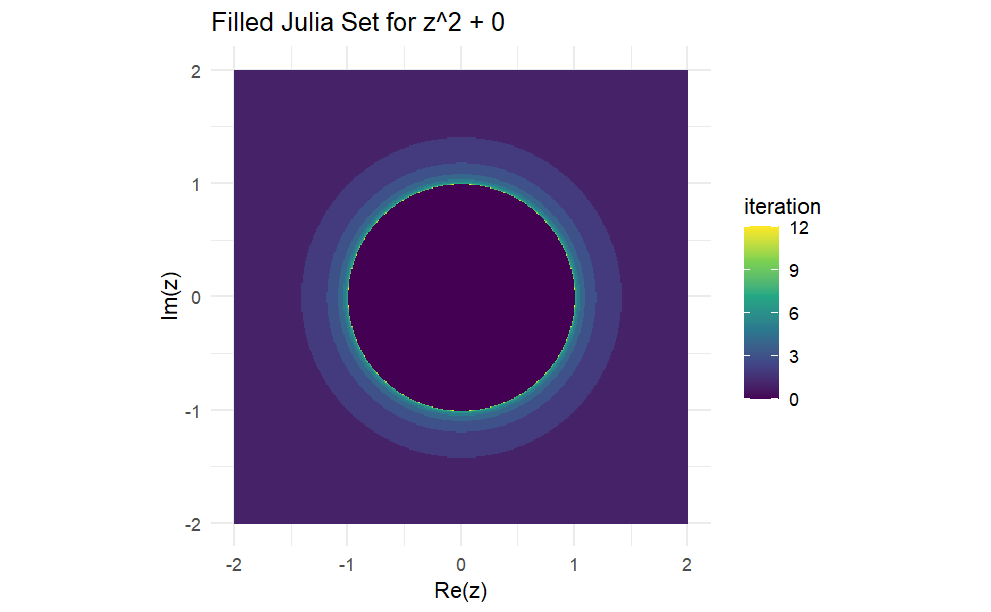
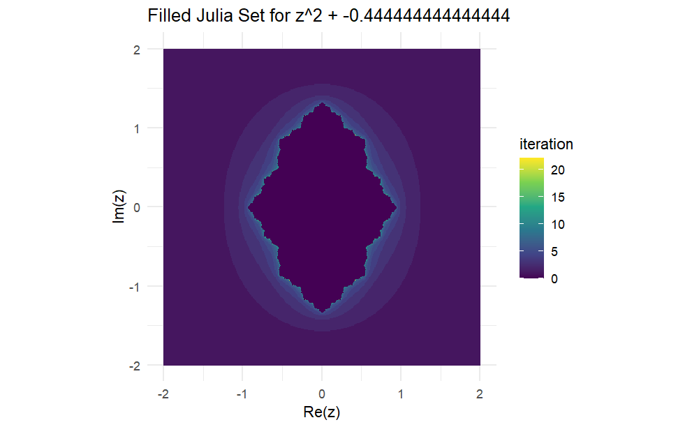
- Visualzation for \(z^2\) & \(f(z) = z^2 - \frac{4}{9}.\)
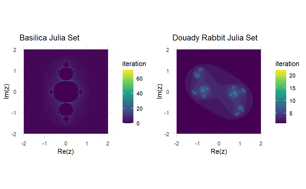
- The Basilica and the Rabbit
- Properties of the Filled Julia Set
- Interactive Animation of Julia Set
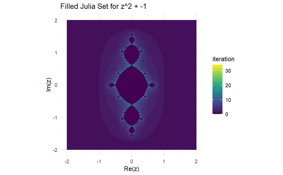
Consider a polynomial map \(f : \mathbb{C} \rightarrow \mathbb{C}\), such as \(f(z) = z^2 - 1\). What are the dynamics of such a map?Certainly, many orbits under this map diverge to infinity:
\[ p_1 = 2, p_2 = 3, p_3 = 8, p_4 = 63, p_5 = 3968, \ldots \]
On the other hand, some orbits manage to remain bounded:
\[ p_1 = 0.5, p_2 = -0.75, p_3 = -0.4375, p_4 \approx -0.8086, \ldots \]
Let \(f : \mathbb{C} \rightarrow \mathbb{C}\) be a polynomial map, and let \(\{p_1, p_2, p_3, \ldots\}\) be an orbit under \(f\).
We say that the orbit is bounded if all the points are contained in some disk of finite radius centered at the origin. That is, the orbit is bounded if there exists a constant ( \(R > 0\) ) so that ( \(|p_n| \leq R\) ) for all \(n \in \mathbb{N}\) .
We say that the orbit escapes to infinity if (\(|p_n| \to \infty\)) as (\(n \to \infty\)).
This leads to the question: for what initial points ( \(p_1\) ) will the orbit under ( \(f\) ) remain bounded, and for what initial points will the orbit escape to infinity?
Let \(f : \mathbb{C} \rightarrow \mathbb{C}\) be a polynomial map.
- The filled Julia set for \(f\) is the set:
\[ {p_1 \in \mathbb{C} | \text{the orbit of } p_1 \text{ is bounded}}. \]
The basin of infinity for ( \(f\) ) is the set:
\[ {p_1 \in \mathbb{C} | \text{the orbit of } p_1 \text{ escapes to infinity}}. \]
Let \(f : \mathbb{C} \rightarrow \mathbb{C}\) be a polynomial function. Let \(B\) be the basin of infinity for \(f\) , and let \(J\) be the filled Julia set for \(f\). Then:
\(B\) and \(J\) are disjoint, and \(B \cup J = \mathbb{C}\).
Both \(B\) and \(J\) are invariant under \(f,\) i.e., \(f(B) = B\) and \(f(J) = J\).
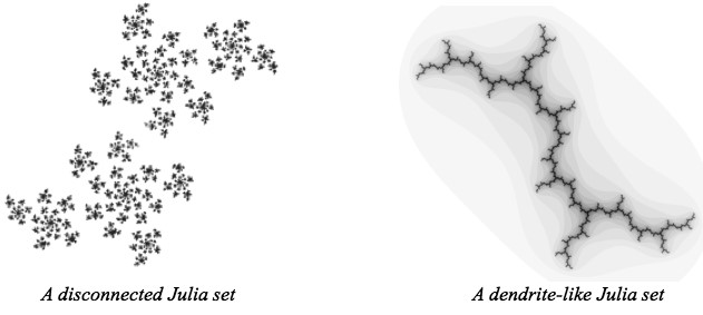
Filled Julia sets can be divided into two categories. Sets are connected so that you can draw a line from one point to another without lifting your pen. Sets where points look like scattered pieces of dust are disconnected.
Iterations & the Mandelbrot Set
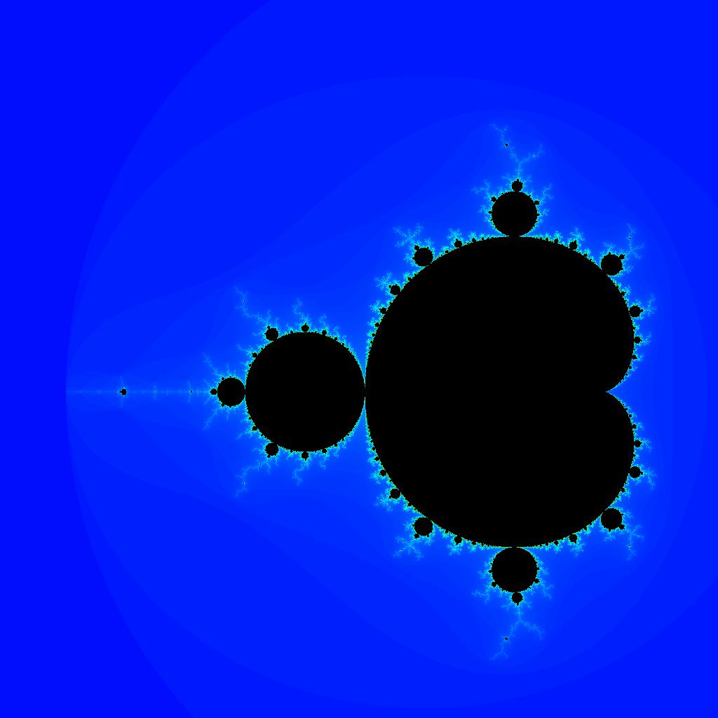
The Mandelbrot set \(M\) is defined in the complex plane as follows:
\[ M = \{ c \in \mathbb{C} \ | \ \text{the sequence defined by } z_{n+1} = z_n^2 + c \text{ with } z_0 = 0 \text{ is bounded} \} \]
Connectedness: The set is connected and exhibits intricate fractal structures.
Boundary: The boundary of the Mandelbrot set is infinitely complex and is where most of the interesting dynamics occur.
The behavior of this sequence determines whether \(c\) is part of the Mandelbrot set:
If the sequence remains bounded, meaning the absolute value of \(z_n\) does not grow beyond a certain limit (typically \(|z| < 2\)), then \(c\) belongs to the Mandelbrot set.
If the sequence diverges, meaning \(z_n\) grows without bound, then \(c\) is not part of the Mandelbrot set.
For example, with \(c = 1\) , the sequence grows rapidly:
\[ z_1 = 1, \quad z_2 = 2, \quad z_3 = 5, \quad z_4 = 26, \ldots \]
showing divergence. However, for \(c = -2\):
\[ z_1 = -2, \quad z_2 = 2, \quad z_3 = 2, \ldots \]
the sequence stabilizes, indicating that \(-2\) is on the boundary of the Mandelbrot set.
The set’s boundary, particularly for real values, lies between \(-2\) and \(\frac{1}{4}\), where points like \(c = -2\) remain bounded, but just beyond \(c = -2.1\), the sequence diverges. This iterative process is key to understanding the fractal structure and complexity of the Mandelbrot set.

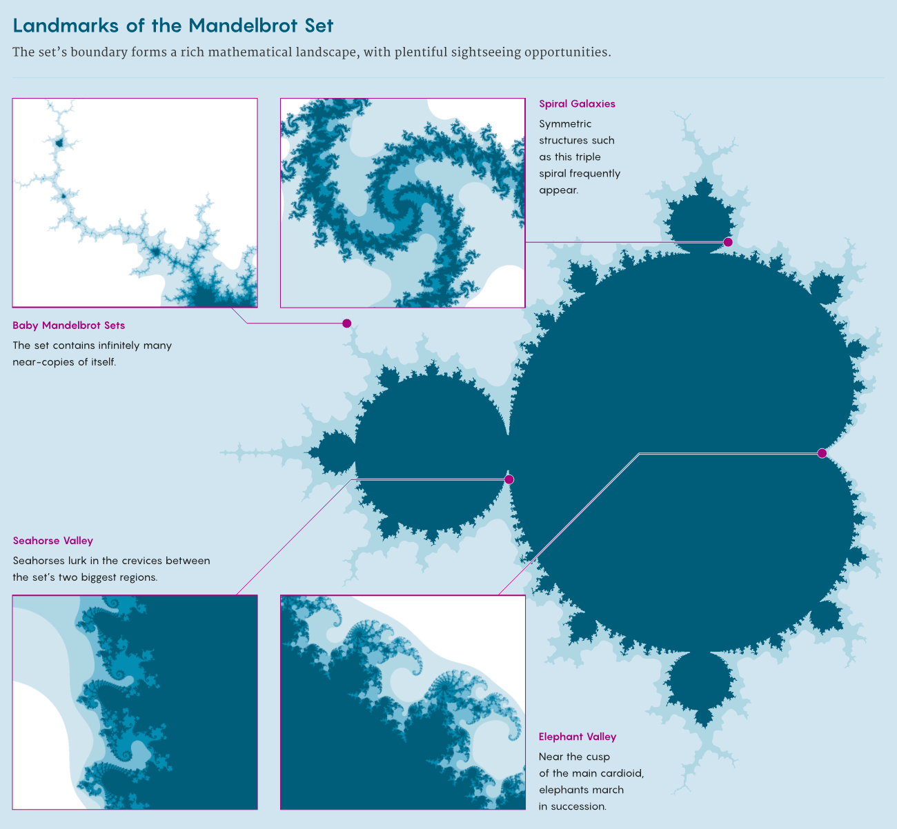
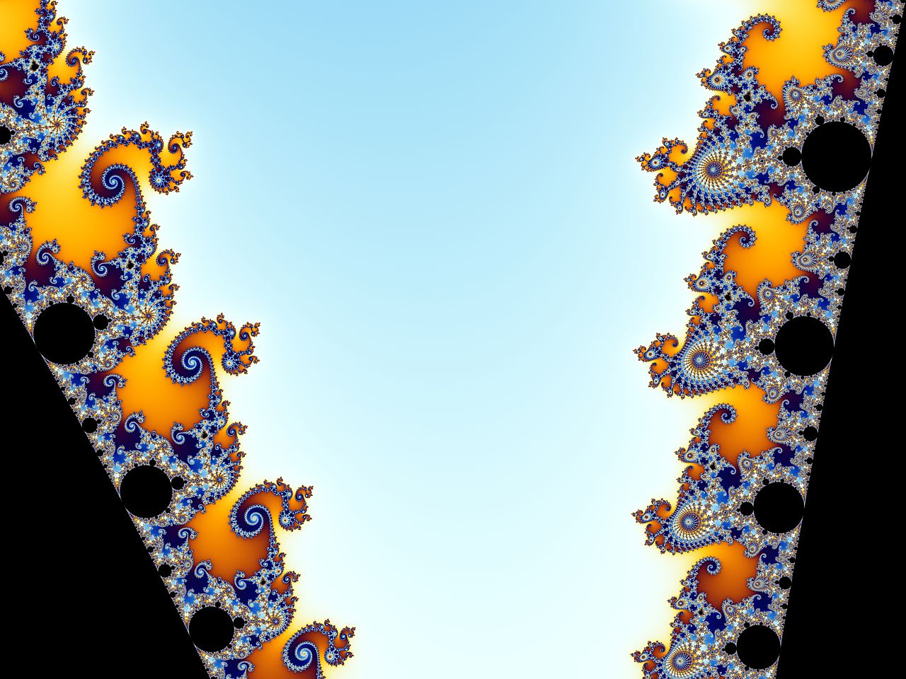
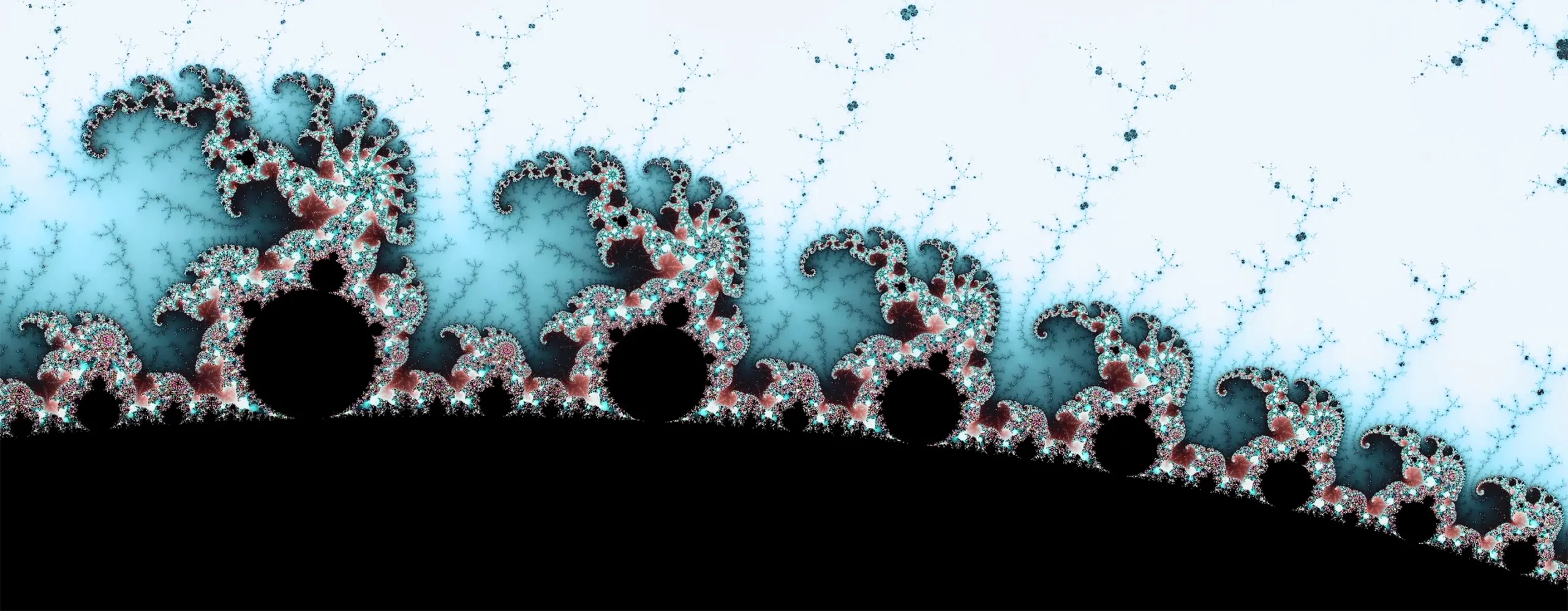
The Mandelbrot set has many intriguing features, but the biggest mysteries lie in its complex fractal boundary. Zooming into different boundary regions reveals some astounding features. A valley of seahorses, parades of elephants and a miniature version of the set itself.