Non-linear Dynamical System (Chaos-Butterfly Effect) using R
Simple Pendulum and Phase Space
A simple pendulum is a mechanical arrangement that demonstrates periodic motion. This non-linear system is periodic ( it repeats itself over and over again at regular intervals ), meaning it follows a repeating pattern. If we start it twice from approximately the same point, we get approximately the same behavior.
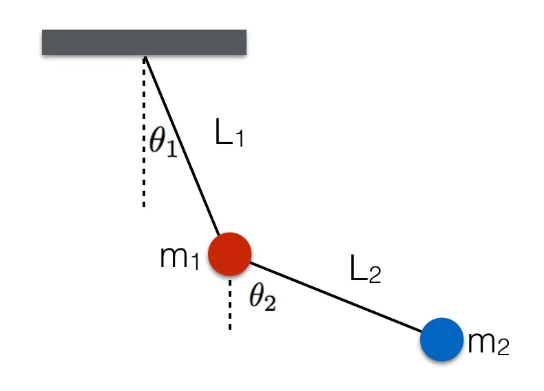
Double Pendulum and Phase Space
Now let’s try two pendulums connected end to end a non-linear system that’s also non-periodic. If we start it twice from approximately the same position, we will get radically different behavior over time.
library(tidyverse)
library(gganimate)
# constants
G  <-  9.807  # acceleration due to gravity, in m/s^2
L1 <-  1.0    # length of pendulum 1 (m)
L2 <-  1.0    # length of pendulum 2 (m)
M1 <-  1.0    # mass of pendulum 1 (kg)
M2 <-  1.0    # mass of pendulum 2 (kg)

parms <- c(L1,L2,M1,M2,G)

# initial conditions
th1 <-  20.0  # initial angle theta of pendulum 1 (degree)
w1  <-  0.0   # initial angular velocity of pendulum 1 (degrees per second)
th2 <-  180.0 # initial angle theta of pendulum 2 (degree)
w2  <-  0.0   # initial angular velocity of pendulum 2 (degrees per second)

state <- c(th1, w1, th2, w2)*pi/180  #convert degree to radians
derivs <- function(state, t){
  L1 <- parms[1]
  L2 <- parms[2]
  M1 <- parms[3]
  M2 <- parms[4]
  G  <- parms[5]

  dydx    <-  rep(0,length(state))
  dydx[1] <-  state[2]

  del_ <-  state[3] - state[1]
  den1 <-  (M1 + M2)*L1 - M2*L1*cos(del_)*cos(del_)
  dydx[2]  <-  (M2*L1*state[2]*state[3]*sin(del_)*cos(del_) +
                  M2*G*sin(state[3])*cos(del_) +
                  M2*L2*state[4]*state[4]*sin(del_) -
                  (M1 + M2)*G*sin(state[1]))/den1

  dydx[3] <-  state[4]

  den2 <-  (L2/L1)*den1
  dydx[4]  <-  (-M2*L2*state[4]*state[4]*sin(del_)*cos(del_) +
                  (M1 + M2)*G*sin(state[1])*cos(del_) -
                  (M1 + M2)*L1*state[2]*state[2]*sin(del_) -
                  (M1 + M2)*G*sin(state[3]))/den2

  return(dydx)
}

library(odeintr)
sol <- odeintr::integrate_sys(derivs,init = state,duration = 30,
                              start = 0,step_size = 0.1)

x1 <-  L1*sin(sol[, 2])
y1 <-  -L1*cos(sol[, 2])

x2 <- L2*sin(sol[, 4]) + x1
y2 <- -L2*cos(sol[, 4]) + y1

df <- tibble(t=sol[,1],x1,y1,x2,y2,group=1)


ggplot(df)+
  geom_segment(aes(xend=x1,yend=y1),x=0,y=0)+
  geom_segment(aes(xend=x2,yend=y2,x=x1,y=y1))+
  geom_point(size=5,x=0,y=0)+
  geom_point(aes(x1,y1),col="red",size=M1)+
  geom_point(aes(x2,y2),col="blue",size=M2)+
  scale_y_continuous(limits=c(-2,2))+
  scale_x_continuous(limits=c(-2,2))+
  ggraph::theme_graph()+
  labs(title="{frame_time} s")+
  transition_time(t) -> p

pa <- animate(p,nframes=nrow(df),fps=20)
pa

tmp <- select(df,t,x2,y2)
trail <- tibble(x=c(sapply(1:5,function(x) lag(tmp$x2,x))),
                y=c(sapply(1:5,function(x) lag(tmp$y2,x))),
                t=rep(tmp$t,5)) %>%
  dplyr::filter(!is.na(x))

library(transformr)
ggplot(df)+
  geom_path(data=trail,aes(group=t,x,y),colour="blue",size=0.5)+
  geom_segment(aes(xend=x1,yend=y1),x=0,y=0)+
  geom_segment(aes( xend=x2,yend=y2,x=x1,y=y1))+
  geom_point(size=5,x=0,y=0)+
  geom_point(aes(x1,y1),col="red",size=M1)+
  geom_point(aes(x2,y2),col="blue",size=M2)+
  scale_y_continuous(limits=c(-2,2))+
  scale_x_continuous(limits=c(-2,2))+
  ggraph::theme_graph()+
  labs(title="{frame_time} s")+
  transition_time(t)+
  shadow_mark(colour="grey",size=0.1,exclude_layer = 2:6)-> p_1
pa_1 <- animate(p_1,nframes=nrow(df),fps=20)
pa_1
Poincare’s Research
In 1903, French mathematician Henri Poincare observed something similar while studying the problem of three objects in space, all affected by each other’s gravity. He was always looking for what’s the most simple set of equations that exhibit chaotic properties. Lorenz found a set of three equations, a simplified version of equations used to model convection, with only three variables that change over time. It is notable for having chaotic solutions for certain parameter values and initial conditions.
Edward Lorenz’s Research
In 1961, Lorenz was working with a set of equations that represented a simplified version of the atmosphere, with 12 variables that changed over time. The computer calculated the values for each moment in time by applying the equations to the values from the previous moment, and Lorenz watched how they progressed. He needed to be sure that like real weather, they did not follow a repeating pattern. In, some cases, Lorenz’s team needed to reprint part of the simulation, so they would restart it from an earlier point by entering the numbers from an earlier printout as start values. Since they used the same numbers and equations, they expected to see the same results.
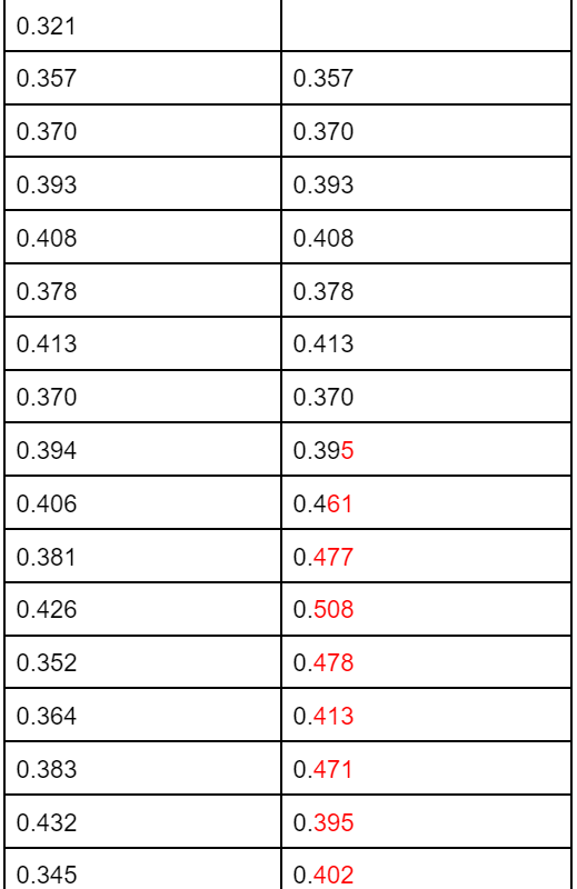
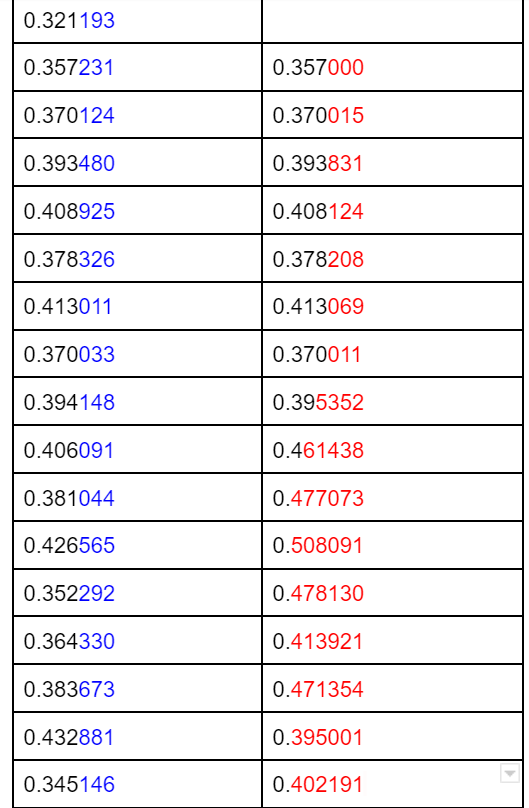
But sometimes they didn’t. In some cases, the second run would look very different from the first as it progressed. At first, Lorenz thought the computer was malfunctioning, but he eventually found the source of the error. While the computer’s memory stores numbers with six decimal places, it printed them with only three decimal places, so the values he entered contained tiny errors. Lorenz was observing that in some systems, tiny changes in the present can lead to big changes in the future.
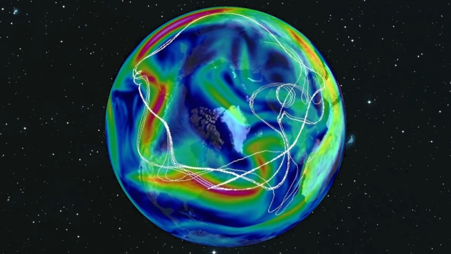
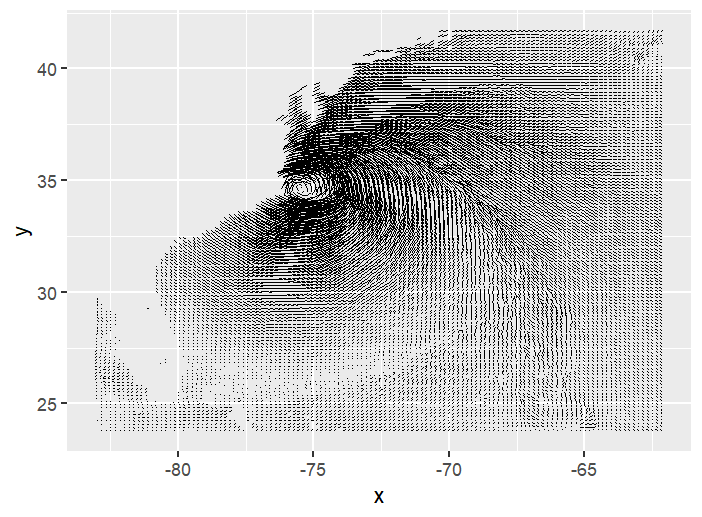
Today we can create models of the atmosphere that go far beyond Lorenz’s columns of numbers. In this model from MIT, the white line represent a bunch of balloons released from approximately the same point. Eventually, the Balloons diverge along very different paths, because of the small differences in their starting points. If you change the initial conditions ever so slightly, infinitesimally slightly. The two trajectories seem to go along with each other and then they diverge exponentially fast. So, that is chaos. It means that you have to know a system with infinite precision to be able to predict it infinitely in time.
Sensitive Dependence on Initial Conditions
When Lorenz entered those initial conditions, the difference of less than one part in a thousand created totally different weather just a short time into the future. Now Lorenz tried simplifying his equations and then simplifying them some more, down to just three equations and three variables that represent the toy model of convection:
\[ \dfrac{dx}{dt}=\sigma(y-x) \]
\[ \dfrac{dy}{dt}=x(\rho-z)-y \]
\[ \dfrac{dz}{dt}=xy-\beta z \]
with the initial conditions : \(x(0)=y(0)=z(0)=1\)
Solving Initial Value Differential Equations in R
1. A Simple ODE: Chaos in the Atmosphere
The Lorenz equations were the first chaotic dynamic system to be described. They consist of three differential equations that were assumed to represent the idealized behavior of the earth’s atmosphere. We use this model to demonstrate how to implement and solve differential equations using R programming. The Lorenz model describes the dynamics of three state variables, \(x,y,\ and\ z\) The model equations are:
\[ \dfrac{dx}{dt}=\sigma(y-x) \]
\[
\dfrac{dy}{dt}=x(\rho-z)-y
\]
\[\dfrac{dz}{dt}=xy-\beta z\]
with the initial conditions : \(x(0)=y(0)=z(0)=1\)
The constants \(\sigma\), \(\rho\), and \(\beta\) are system parameters proportional to the Prandtl number, Rayleigh number, and certain physical dimensions of the layer itself where \(\sigma\), \(\rho\), and \(\beta\) are three parameters, with values of\(\sigma = 10,\ \beta= \frac{8}{3}, \rho=28\). Implementation of an IVP ODE in R can be separated into two parts: ‘the model specification’ and the ‘model application’.
The model specification consists of:
• Defining model parameters and their values,
• Defining model state variables and their initial conditions,
• Implementing the model equations that calculate the rate of change (e.g. \(\frac{dx}{dt}\)) of the state variables.
The model application consists of:
• Specification of the time at which model output is wanted,
• Integration of the model equations (uses R-functions from deSolve),
• Plotting of model results.
1.1. MODEL SPECIFICATION
Model parameters:
There are three model parameters: s, r, and b that are defined first. Parameters are stored as a vector with assigned names and values:
parameters <- c(s=10,r=28,b=8/3)State Variables:
The three state variables are also created as a vector, and their initial values are given:
initial_state <-
  c(x = -8.60632853,
    y = -14.85273055,
    z = 15.53352487)
Model Equation
The model equations are specified in a function (Lorenz) that calculates the rate of change of the state variables. Input to the function is the model time (t, not used here, but required by the calling routine), and the values of the state variables (state) and the parameters, in that order. This function will be called by the R routine that solves the differential equations (here we use ode, see below). The code is most readable if we can address the parameters and state variables by their names. As both parameters and state variables are ‘vectors’, they are converted into a list. The statement with (as. list (c(state, parameters)), …) then makes available the names of this list. The main part of the model calculates the rate of change of the state variables. At the end of the function, these rates of change are returned, packed as a list. Note that it is necessary to return the rate of change in the same ordering as the specification of the state variables. This is very important. In this case, as state variables are specified \(x\) first, then \(y\) and \(z\), the rates of changes are returned as \(dx,dy,dz\).
lorenz <- function(t, state, parameters) {
  with(as.list(c(state, parameters)), {
    dx <- sigma * (y - x)
    dy <- x * (rho - z) - y
    dz <- x * y - beta * z

    list(c(dx, dy, dz))
  })
}
1.2. MODEL APPLICATION:
Time Specification
We run the model for 100 days, and give output at 0.01 daily intervals. R’s function seq( ) creates the time sequence:
times <- seq(0, 500, length.out = 125000)Model Integration
The model is solved using ’deSolve’ function ode, which is the default integration routine. Function ode takes as input, a.o. the state variable vector (y), the times at which output is required (times), the model function that returns the rate of change (func) and the parameter vector (parms). Function ode returns an object of class deSolve with a matrix that contains the values of the state variables (columns) at the requested output times.
lorenz_ts <-
  ode(
    y = initial_state,
    times = times,
    func = lorenz,
    parms = parameters,
    method = "lsoda"
  ) %>% as_tibble()

lorenz_ts[1:10,]
Plotting Results:
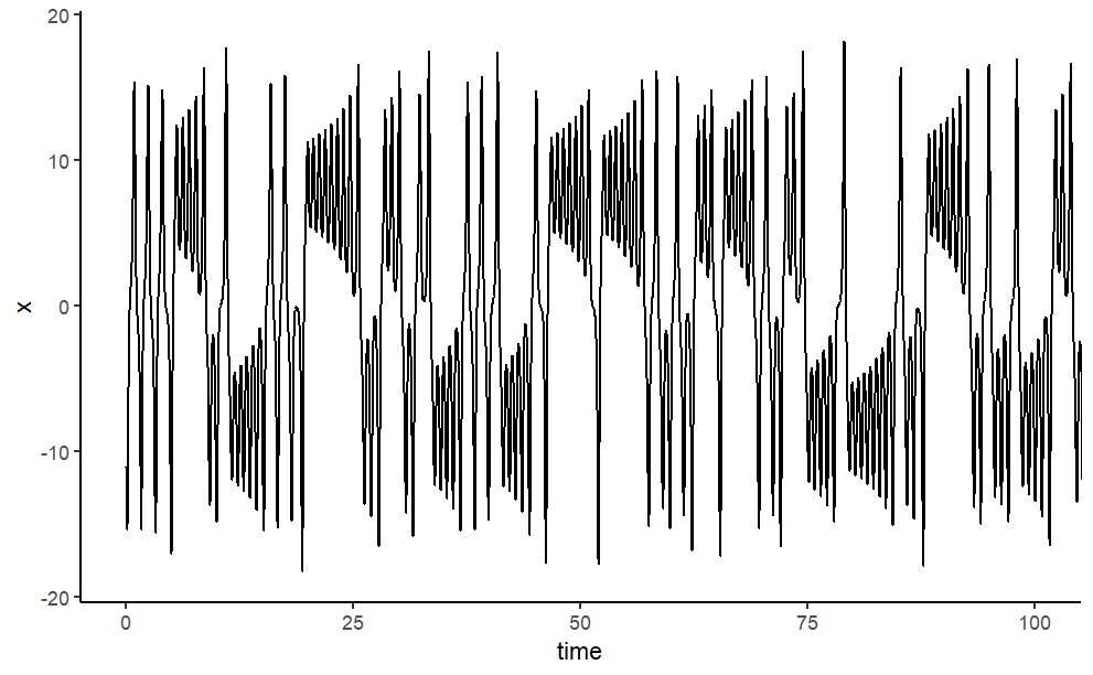
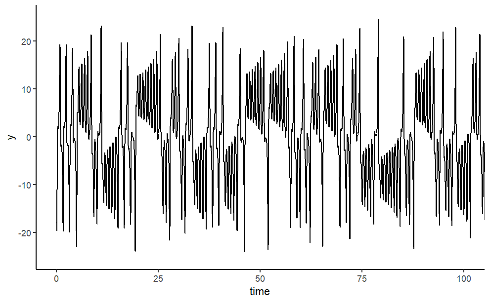
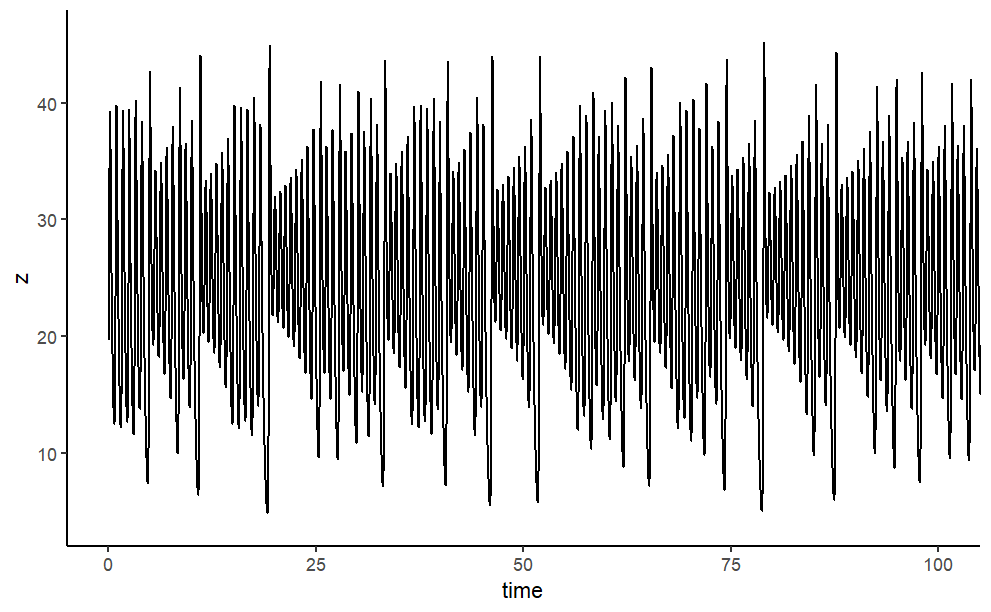
Finally, the model output is plotted. We use the plot method designed for objects of class deSolve, which will neatly arrange the figures in two rows and two columns; before plotting, the size of the outer upper margin (the third margin) is increased. We access to \(x\),\(y\),\(z\) respectively a univariate time series. As the time interval used to numerically integrate the differential equations was rather tiny, we just use every tenth observation.
essentially a 2d slice of the atmosphere heated at the bottom and cooled at the top. But again, he got the same type of behavior; if he changed the numbers just a tiny bit, results diverged dramatically.
Lorenz’s system displayed what’s become known as the sensitive dependencies on initial time conditions, which is the hallmark of chaos. Now since Lorenz was working with three variables, we can plot the phase space of his system in three dimensions. We can pick any points as our initial state and watch how it evolves.
Experimentation using R
Iteration Using sapply( ) Function
We want to calculate the sequence \(x_{n+1} =cos(x_n)\) for 100 steps.
Iteration Reaches a Bizarre Value
The latter relation belongs to the family of one-dimensional maps and we can describe its behavior as a damped oscillation that converges to the stable value, of ~\(0.739\). This value is the solution to the transcendental equation \(x=cos(x)\).
#get random angle
set.seed(1)
random_angle  <- sample(seq(1, 2*pi, length.out = 100), 1)
#start from here
get_value <- cos(random_angle)
n_steps <- seq(100)
#perfome iteration 150 times
bizarre_sequence <-
  sapply(n_steps, function(x){
    get_value <<- cos(get_value)
  })
#get convergence/last value
tail(bizarre_sequence, 1)
library(tidyverse)
ggplot() +
  geom_line(aes(x = n_steps, y = bizarre_sequence)) +
  ylab(expression('cos x'[n])) +
  xlab("n")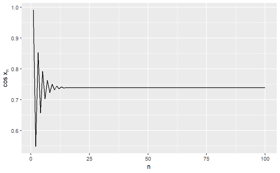
Chaotic Behavior Due to Changes in Parameter
Let’s do some calculations for a range of the \(r\) parameter \(1.5≤r≤2.9\) and see how the system behaves. In particular, we will calculate a sequence for nine distinct values of \(r\) and to inspect the behavior of the system for the nine different values of \(r\) we will plot the values of the sequences faceting on \(r\).
library(dplyr)
library(data.table)
set.seed(11)
getbizarre_sequences <- function(r, n_steps = 100){
  #get random angle
  random_angle  <- sample(seq(1, 2*pi, length.out = 100), 1)
  #get cos value
  get_value <- cos(random_angle)
  dt <-
    sapply(seq(n_steps), function(x){
      get_value <<- r * cos(get_value)
    }) %>% data.table

  dt[ , n := seq(n_steps)]

}

r_range <- seq(from = 1.5, to = 2.9, length.out = 9)

#calculating sequences
bizarre_list <- lapply(r_range, getbizarre_sequences)
names(bizarre_list) <- paste("r =", r_range)
#tidying data to long range
bizarre_sequences <- rbindlist(bizarre_list, idcol = TRUE)
#View(bizarre_sequences)

library(kableExtra)
dt <- bizarre_sequences[ , head(.SD, 3), by = .id]
kable(dt %>% head)

ggplot(bizarre_sequences, aes(x = n, y = ., group = .id)) +
  geom_line() +
  ylab(expression('r cos x'[n])) +
  xlab("n") +
  facet_wrap( ~ .id, ncol = 3)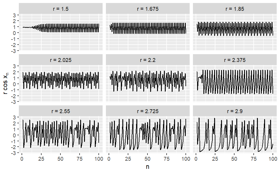
The above diagram depicts the transition of the system between chaotic and ordered phases as r changes. From the previous analysis, we can safely conclude that the system may rest to a stable fixed point \((r=1)\), may enter a cyclic behavior \((r=1.5)\), or a chaotic phase \((r = 2.75)\). The critical values of \(r\) that the system changes state between stable, static, and chaotic behavior due to changes in the parameters of the system are known as bifurcations.
Bifurcation Diagram
As we have just seen changes in the parameters, produce some strange patterns for \(1.5≤r≤2.9\). Let’s study this phenomenon more rigorously. To do so we will study hundreds of different values for \(r\), all between \(1.5\) and \(2.9\), and examine which values of \(x\) the system eventually settles. To identify this state transition, let the system evolve for a considerable amount of iterations and collect the tail of the sequence generated. This process is repeated for a range of \(r\).
r_range <- seq(from = 1, to = 3, length.out = 1000)

bizarre_list <-
  lapply(r_range, function(x){
    tail(getbizarre_sequences(x, n_steps = 10000), 3000)
  })
names(bizarre_list) <- r_range
bizarre_sequences <- rbindlist(bizarre_list, idcol = TRUE)

bizarre_sequences[, .(r = as.numeric(.id), y = .)] %>%
  ggplot(aes(x = r, y = y)) +
  geom_point(size = 0.01, alpha = 0.01) +
  theme_light()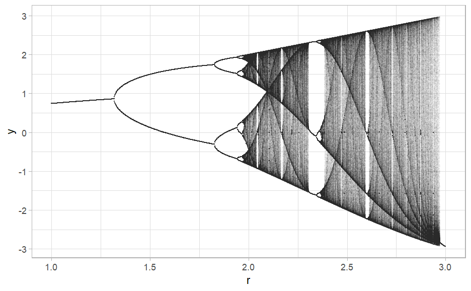
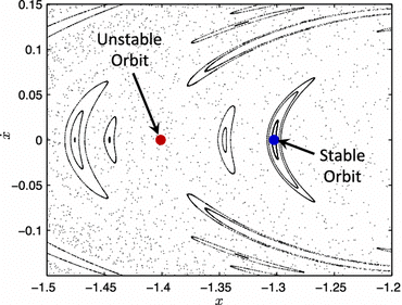
Phase Space or State Space
As a result, there’s a very convenient geometrical and visual way of representing a dynamical system known as the phase space or state space.
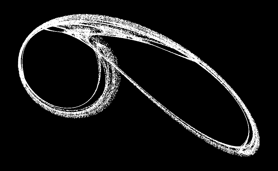
Two Famous Attractor
One of the most prominent strange attractors based on a quadratic map is the so-called Hénon map named after French mathematician Michel Hénon. The Hénon map is typically written as
\[x_{t+1}=1-ax^2_t+y_t\]
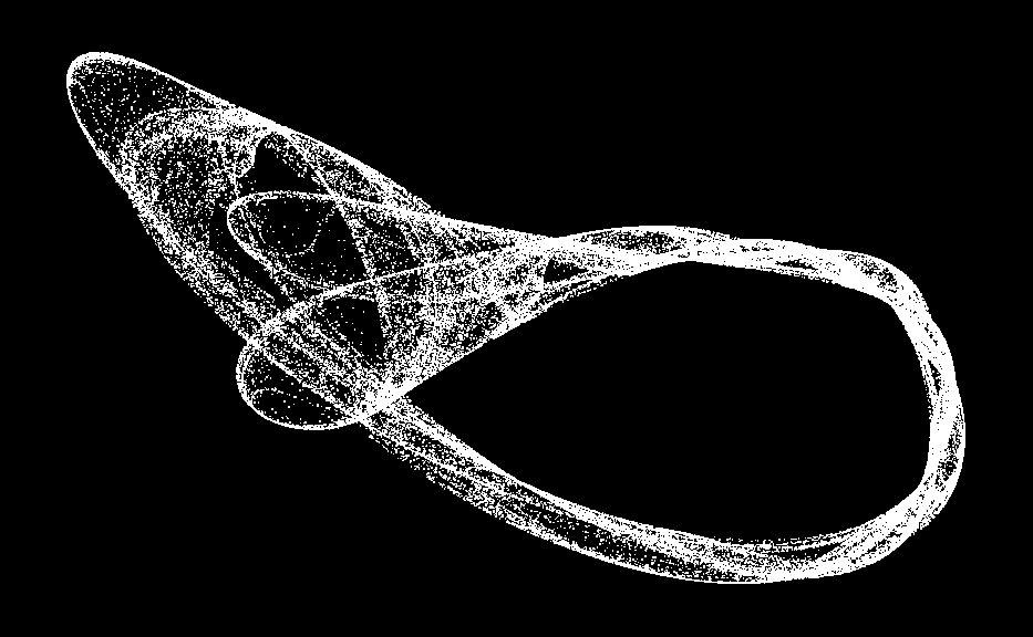
\[y_{t+1}=bx_t\]with \(a=0.9\) and \(b=0.3\). Another well-known chaotic quadratic map is the Tinkerbell map, which is commonly written as,
\[x_{t+1} = ax_t+by_t+x^2_t-y^2_t\]
\[ y_{t+1} = cx_t+dy_t+2x_ty_t \]with \(a=0.9, b=−0.6013, c=2\ and\ d=0.5\). Now, all we need to do is to substitute these coefficients into equations (1),(2) and we are ready to plot the first of many hypnotic images. As we programmed different coloring options into our plot function, we can even produce plots with different colors.
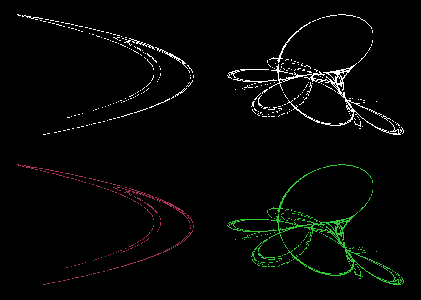
Our Own Strange Attractors
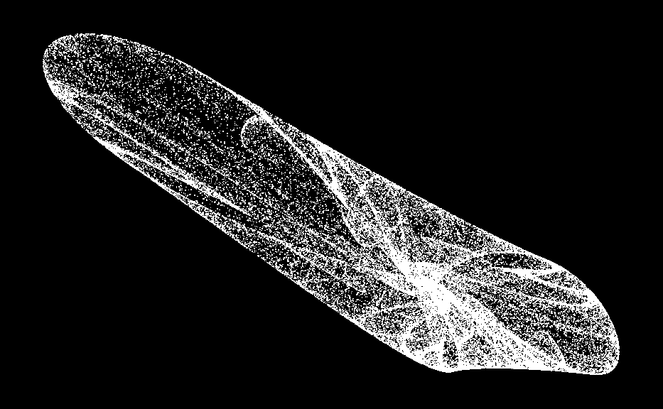
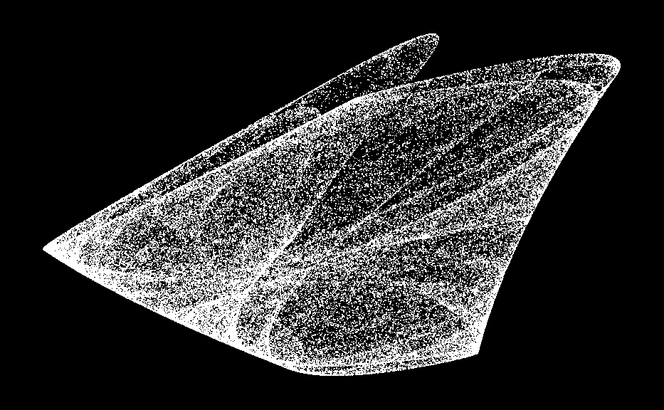
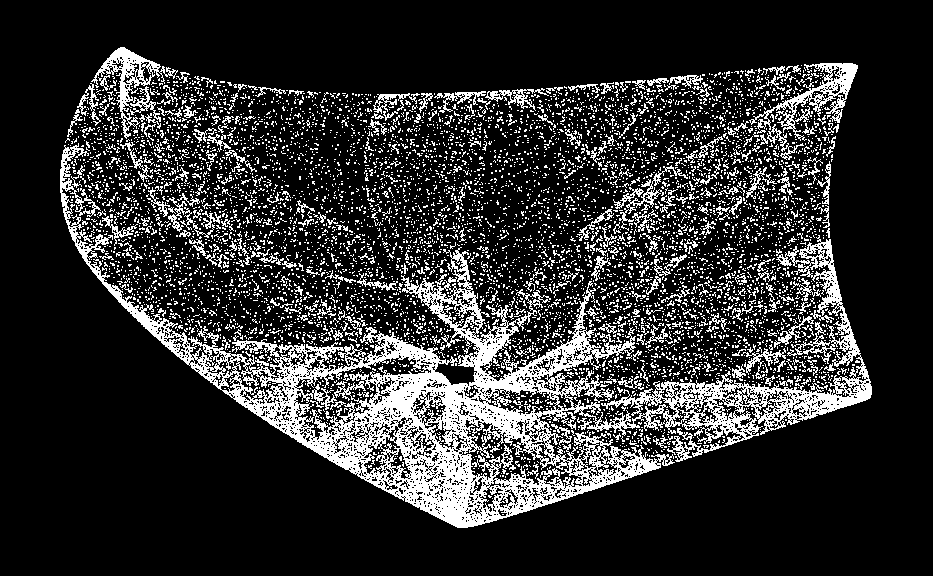

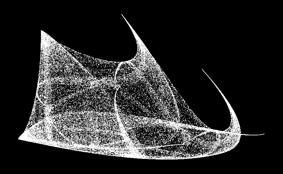
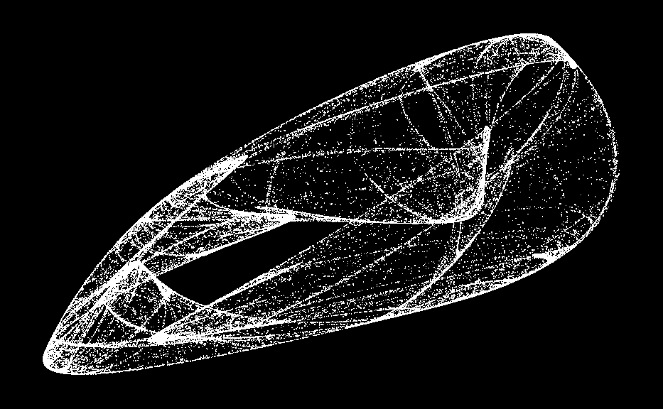
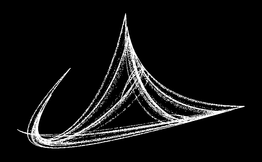
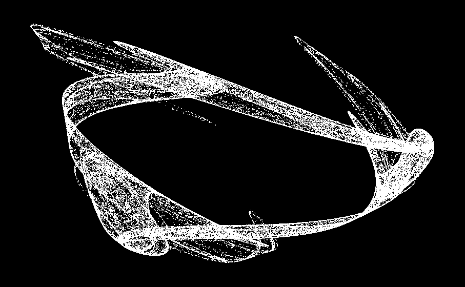
Trajectories are just curves
Trajectories are just curves, so they should be 1-dimensional. But how come no matter how much you zoom in on this attractor, you can always find more and more trajectories everywhere?
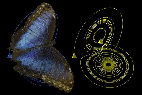
Butterfly Effect: A Metaphor
This was the major challenge to the idea of the Cartesian Universe. The whole idea that certain systems have these finite prediction horizons that you can’t go beyond which was really new. Nobody imagined that to be the case. When Lorenz presented this work at a conference in 1972, the organizer didn’t receive his talk title in time, so he suggested one:
“Does the flap of a butterfly’s wings in Brazil set off a Tornado in Texas?”
In 1987, a popular book by James Gleick introduced the world to the work of Lorenz and other Chaos pioneers, and the ‘Butterfly Effect’ became part of popular culture.

Beautiful Structure Underlying Dynamics