In the dim glow of the computer screen, our protagonists sat mesmerized by the hypnotic dance unfolding before them. Lines twisted and turned, forming intricate patterns that seemed to pulse with a life of their own. This wasn’t just any digital artwork; it was the manifestation of a mathematical marvel known as the Clifford attractor.
But how did our protagonists find themselves immersed in this captivating world of chaos and beauty?
It all began one rainy afternoon, as they stumbled upon an old book tucked away in the dusty corner of a library. Its pages whispered tales of strange attractors, chaotic systems that defied predictability yet exuded a haunting allure. Intrigued, our protagonist embarked on a journey of exploration, armed with nothing but curiosity and a genuine desire to unravel the mysteries of chaos.
What Are Strange Attractors?
In math, a dynamical system tells us how a point in space changes over time using some fancy functions. An attractor is like a magnetic force that pulls points toward certain values over time, no matter where they start from. Simple attractors are kind of like fixed points or loops that the system settles into. But things get interesting with strange attractors. They’re like wild, unpredictable whirlpools in math space where the system can roam around without repeating itself.
One of the most famous strange attractors, discovered by this person named Kiyohiro Ikeda, is named after him. It’s all described by these equations:
\[
x_{n+1}= 1+u(x_n \cos t_n −y_n \sin t_n)
\]
\[
y_{n+1} = u (x_n \sin t_n + y_n \cos t_n)
\]
with \(u ≥ 0.6\) and
\[
t_n = 0.4 − \dfrac{6}{1+ x_n^2 + y^2_n}
\]
In this example, our imaginary point moves in a 2D-dimensional space, since we just need (x, y) coordinates to describe its movement. In the previous system, time is represented by n. As you can see, Ikeda’s system only depends on one parameter, called u. The location of the point at n depends only on its location at n-1. For example, this image shows the trajectories of \(2000\) random points following this previous equation with \(u=0.918\):
Code
u=0.918#Parameter between 0 and 1n=2000#Number of particlesm=40#Number of iterationsikeda=data.frame(it=1,x1=runif(n, min =-40, max =40), y1=runif(n, min =-40, max =40))ikeda$x2=1+u*(ikeda$x1*cos(0.4-6/(1+ikeda$x1^2+ikeda$y1^2))-ikeda$y1*sin(0.4-6/(1+ikeda$x1^2+ikeda$y1^2)))ikeda$y2= u*(ikeda$x1*sin(0.4-6/(1+ikeda$x1^2+ikeda$y1^2))+ikeda$y1*cos(0.4-6/(1+ikeda$x1^2+ikeda$y1^2)))for (k in1:m){df=as.data.frame(cbind(rep(k+1,n),ikeda[ikeda$it==k,]$x2,ikeda[ikeda$it==k,]$y2,1+u*(ikeda[ikeda$it==k,]$x2*cos(0.4-6/(1+ikeda[ikeda$it==k,]$x2^2+ikeda[ikeda$it==k,]$y2^2))-ikeda[ikeda$it==k,]$y2*sin(0.4-6/(1+ikeda[ikeda$it==k,]$x2^2+ikeda[ikeda$it==k,]$y2^2))),u*(ikeda[ikeda$it==k,]$x2*sin(0.4-6/(1+ikeda[ikeda$it==k,]$x2^2+ikeda[ikeda$it==k,]$y2^2))+ikeda[ikeda$it==k,]$y2*cos(0.4-6/(1+ikeda[ikeda$it==k,]$x2^2+ikeda[ikeda$it==k,]$y2^2)))))names(df)=names(ikeda)ikeda=rbind(df, ikeda)}plot.new()par(mai =rep(0, 4), bg ="gray12")plot(c(0,0),type="n", xlim=c(-35, 35), ylim=c(-35,35))apply(ikeda, 1, function(x) lines(x=c(x[2],x[4]), y=c(x[3],x[5]), col =paste("gray", as.character(min(round(jitter(x[1]*80/(m-1)+(20*m-100)/(m-1), amount=5)), 100)), sep =""), lwd=0.1))
All points, regardless of their starting place, tend to end following the same path, represented in bright white colour. Another interesting property of strange attractors is that points that are very close at some instant, can differ significantly in the next step. This is why strange attractors are also known as chaotic attractors.
Clifford Attractor’s Mathematical Construction
Understanding the Clifford attractor was no easy feat. Its equations danced on the edge of complexity, teasing our protagonist with their elusive secrets. As they delved deeper into its mathematical underpinnings, our protagonist discovered a world of recursive equations and chaotic trajectories. The Clifford attractor, named after its creator Clifford A. Pickover, was no ordinary mathematical construct. It was a window into the unpredictable nature of dynamical systems, where order emerged from chaos in the most unexpected ways. Now, we will experiment with Clifford attractors, but before diving into the experiment first we’ll introduce this attractor formally.
Formalism
A Clifford Attractor is a strange attractor defined by two iterative equations that determine the \(x,y\) locations of discrete steps in the path of a particle across a 2D space, given a starting point \((x_0,y_0)\) and the values of four parameters \((a,b,c,d)\):
\[
x_{n+1} = \sin
(ay_n) + c \cos (ax_n)
\]
\[
y_{n+1} = \sin(b x_n) +d \cos(by_n)
\]
At each time step, the equations define the location for the following time step, and the accumulated locations show the areas of the 2D plane most commonly visited by the imaginary particle.
Unlocking Efficiency
Populating Attractors
The Clifford attractor is a mathematical concept that falls under the broader category of Strange Attractors. It’s a type of chaotic dynamical system that exhibits complex and beautiful patterns when iterated through a set of equations. The computational approach to exploring the Clifford attractor involves implementing these equations in code to visualize the attractor’s behaviour.
The Power of Iteration in Programming
Iteration lies at the heart of every programming language, serving as an indispensable technique for crafting robust, speedy, and concise code. It’s the art of repeating tasks over and over, streamlining complex operations into manageable sequences. At its core lies the humble loop, a programming construct that condenses numerous lines of code into a compact, efficient form. By mastering iteration, programmers gain the ability to tackle daunting tasks with ease. With each loop iteration, they chip away at computational challenges, forging elegant solutions that are both powerful and succinct. Whether it’s processing vast datasets or executing intricate algorithms, iteration empowers programmers to navigate complexity with finesse.
In the realm of software development, efficiency is key. Writing efficient loops not only optimizes performance but also enhances code readability and maintainability. It allows developers to express their logic concisely, making it easier for others to understand and modify the code in the future. Indeed, the significance of iteration extends far beyond mere repetition. It embodies the essence of problem-solving in programming, enabling developers to transform abstract concepts into tangible solutions. As programmers harness the power of iteration, they unlock new realms of possibility, paving the way for innovation and discovery in the ever-evolving landscape of technology.
Strange Attractors: An R Experiment
Recursivity & Creative Coding
Learning to code can be quite hard. Apart from the difficulties of learning a new language, following a book can be quite boring. One of the best ways to become a good programmer is to choose small and funny experiments oriented to training specific techniques of programming. In this tutorial, we will learn to combine C++ with R to create efficient loops. We will also learn interesting things about ggplot2, a very important package for data visualization. The excuse to do all this is to create beautiful images using a mathematical concept called Strange Attractors, which we will discuss briefly also. Combining art and coding is often called generative art, so be ready because after following this tutorial you can discover a new use of R to fall for as I am. Here we go!
In R, you can do this using the for() function. For example, this loop calculates the mean of each column of a data frame called df() :
Code
library(tidyverse)n <-1000# Rows of data frame# df with 4 columns and n rows sampled from N(0,1)df <-tibble(a =rnorm(n),b =rnorm(n),c =rnorm(n),d =rnorm(n))output <-vector("double", ncol(df)) # Empty output# For loopfor (i in1:ncol(df)) { output[[i]] <-mean(df[[i]])}output
In the previous example, we repeated 4 times the task (which is the piece of code inside the curly brackets). Another way to do iterations in R, sometimes more efficient than a for loop, is by using the apply family. This is how the previous loop can be rewritten using the apply() function:
Code
output <-apply(df, 2, mean)output
These approaches have limitations. For example, if you want to use the result of an iteration as the input of the next one, you can not use apply. Another one is that sometimes R is not enough fast, which makes the for function quite inefficient. When you face this kind of situation, a good option is combining C++ and R.
To represent the trajectory of a particular point, we need to store in a data frame its locations at every single (discrete) moment. For example, this is how we can do it using a for loop:
Code
# Parameters settinga <--1.25b <--1.25c <--1.82d <--1.91# Number of jumpsn <-5# Initialization of df to store locations of pointdf <-data.frame(x =double(n+1), y =double(n+1))# The point starts at (0,0)df[1, "x"] <-0df[1, "y"] <-0# For loop to store locationsfor (i in1:n) { df[i+1, "x"] <-sin(a*df[i, "y"])+c*cos(a*df[i, "x"]) df[i+1, "y"] <-sin(b*df[i, "x"])+d*cos(b*df[i, "y"])}df
           x          y
1  0.0000000  0.0000000
2 -1.8200000 -1.9100000
3  1.8629450  2.1543131
4  0.8172482  0.9946399
5 -1.8969558 -1.4673201
6  2.2716156  1.1936322
As you can see, our point started at \((0,0)\) and jumped \(5\) times (the number of jumps is represented by \(n\)). You can try to change \(n\) from \(5\) to \(10000000\) and see what happens (disclaimer: be patient). A better approach to do it is using purrr, a functional programming package which provides useful tools for iterating through lists and vectors, generalizing code and removing programming redundancies. The purrr tools work in combination with functions, lists and vectors and results in code that is consistent and concise. This can be a purrr approach to our problem:
Code
library(purrrlyr)n <-5# Initialization of our data framedf <-tibble(x =numeric(n+1),y =numeric(n+1))# Convert our data frame into a listby_row(df, function(v) list(v)[[1L]], .collate ="list")$.out -> df# This function computes current location depending of previous onef <-function(j, k, a, b, c, d) {tibble(x =sin(a*j$y)+c*cos(a*j$x),y =sin(b*j$x)+d*cos(b*j$y) )}# We apply accumulate on our list to store all steps and convert into a data frameaccumulate(df, f, a, b, c, d) %>%map_df(~ .x) -> dfdf
# A tibble: 6 × 2
       x      y
   <dbl>  <dbl>
1  0      0
2 -1.82  -1.91
3  1.86   2.15
4  0.817  0.995
5 -1.90  -1.47
6  2.27   1.19
Even this approach is not efficient since the accumulate() function must be applied on an existing object (the df() in our case)
Combining C++ and R
The paragraph below extracted from Hadley Wickham’s Advanced R, explains the motivations of combining C++ and R:
Rcpp makes it very simple to connect C++ to R and provides a clean, approachable API that lets you write high-performance code, insulated from R’s complex C API. Typical bottlenecks that C++ can address include:
Loops that can’t be easily vectorised because subsequent iterations depend on previous ones.
Recursive functions, or problems which involve calling functions millions of times. The overhead of calling a function in C++ is much lower than in R.
Problems that require advanced data structures and algorithms that R doesn’t provide. Through the standard template library (STL), C++ has efficient implementations of many important data structures, from ordered maps to double-ended queues.
This code populates our data frame using C++:
Code
# Load in libarieslibrary(Rcpp)library(tidyverse)# Here comes the C++ codecppFunction('DataFrame createTrajectory(int n, double x0, double y0, double a, double b, double c, double d) { // create the columns NumericVector x(n); NumericVector y(n); x[0]=x0; y[0]=y0; for(int i = 1; i < n; ++i) { x[i] = sin(a*y[i-1])+c*cos(a*x[i-1]); y[i] = sin(b*x[i-1])+d*cos(b*y[i-1]); } // return a new data frame return DataFrame::create(_["x"]= x, _["y"]= y); } ')a <--1.25b <--1.25c <--1.82d <--1.91# Call the function starting at (0,0) to store 10M jumpsdf <-createTrajectory(10000000, 0, 0, a, b, c, d)head(df)
Note that, apart from Rcpp, we also loaded the tidyverse package. This is because we will use some of its features, as dplyr or ggplot2, later.
The function createTrajectory() is written in C++ and stores the itinerary of an initial point. You can try it to see that It’s extremely fast. In the previous example, I populated on the fly our data frame with 10 million points starting at \((0,0)\) in less than 5 seconds in a conventional laptop.
Rendering the Plot with ggplot()
Once we have built our data frame, it’s time to represent it with ggplot(). Making graphics is a necessary skill and for this ggplot() is an amazing tool, which by the way, I encourage you to learn. Usually, a good visualization is the best way to show your results. R is an extraordinary tool for visualizing data and one of the most important libraries to do it is ggplot2: it is powerful, flexible and is updated to include functionalities regularly. Although its syntax may seem a bit strange at first, here are four important concepts from my point of view to help you out with understanding it:
It’s truly important to have clear the type of graph you want to plot: for each one there’s a different geometry: geom_point to represent points, geom_line to represent time series, geom_bar to do bar chars … Have a look to ggplot2 package, there are many other types.
Each of those geometries needs to define what data is to be used and how. For example, as you will see in our graph, we placed on the x-axis the x column of our data frame df and y on the y-axis, so we did aes(x = x, y = y).
You can also combine geometries. We didn’t do that for our example but you may want, for example, to combine bars and lines on the same plot. To do it you can just use + operator. This operator is very important: it doesn’t only combine geometries, it’s also used to add features to the plot as we did to define its aspect ratio (with coord_equal) or its appearance (with theme_void).
You can modify every detail of the look and feel of your graph but be patient. To begin with, I recommend the use of predefined themes as I did with theme_void. There are many of them and it’s is a quick and easy way to change the appearance of your plot: just a way of making life easier and simpler.
The ggplot2 package is a new world by itself and takes part of the tidyverse, a collection of efficient libraries designed to analyze data in a consistent way. This is how we can represent the points of our data frame:
library(Rcpp)library(ggplot2)library(dplyr)opt =theme(legend.position ="none",panel.background =element_rect(fill="white"),axis.ticks =element_blank(),panel.grid =element_blank(),axis.title =element_blank(),axis.text =element_blank())cppFunction('DataFrame createTrajectory(int n, double x0, double y0, double a, double b, double c, double d) { // create the columns NumericVector x(n); NumericVector y(n); x[0]=x0; y[0]=y0; for(int i = 1; i < n; ++i) { x[i] = sin(a*y[i-1])+c*cos(a*x[i-1]); y[i] = sin(b*x[i-1])+d*cos(b*y[i-1]); } // return a new data frame return DataFrame::create(_["x"]= x, _["y"]= y); } ')a=-1.24458046630025b=-1.25191834103316c=-1.81590817030519d=-1.90866735205054df=createTrajectory(10000000, 0, 0, a, b, c, d)png("Clifford.png", units="px", width=1600, height=1600, res=300)ggplot(df, aes(x, y)) +geom_point(color="black", shape=46, alpha=.01) + optdev.off()
particularly using Rcpp to incorporate C++ code within R, lies in its efficiency and versatility:
Efficiency: By leveraging C++ through Rcpp, computationally intensive tasks can be executed much faster compared to pure R code. C++ is known for its performance, making it ideal for handling large data sets or complex calculations.
Versatility: Integrating C++ code within R expands the capabilities of the R language. It allows developers to access C++ libraries and functionalities, enabling them to implement advanced algorithms or optimize existing code for better performance.
Ease of Use: Despite the complexity of C++, Rcpp simplifies the process of incorporating C++ code within R scripts. Developers can write C++ functions directly within their R environment, avoiding the need for separate compilation and linking processes.
Interoperability: The resulting code is seamlessly integrated with R, allowing users to interact with C++ functions just like any other R function. This interoperability facilitates collaboration and code reuse within the R ecosystem.
Graphics and Visualization: The code snippet demonstrates the seamless integration of C++ computations with R’s powerful visualization capabilities, particularly with ggplot2. This combination enables users to analyze and visualize data efficiently, enhancing the interpretability of results.
Scalability: With C++ optimization, code performance scales efficiently with increasing dataset sizes. This scalability is crucial for handling large-scale data analysis tasks commonly encountered in research, industry, and data science applications.
The syntax of our plot is quite simple. Just two comments about it:
Shape is set to \(46\), the smallest filled point. More info about shapes, here
Since there are a lot of points, I make them transparent with alpha to take advantage on its overlapping and reveal patterns of shadows.
Playing with Parameters
Strange attractors are extremely sensitive to their parameters. This feature makes them very entertaining as well as an infinite source of surprises. This is what happens to Clifford attractor when setting a, b, c and d parameters to -1.2, -1.9, 1.8 and -1.6 respectively:
Code
a <--1.2b <--1.9c <-1.8d <--1.6df <-createTrajectory(10000000, 0, 0, a, b, c, d)ggplot(df, aes(x = x, y = y)) +geom_point(shape =46, alpha = .01) +coord_equal() +theme_void() -> plotggsave("strange2.png", plot, height =5, width =5, units ='in')
Don’t you feel like playing with parameters? From my point of view, this is a very classy way of spending your time.
The General 2D-Map
Once we know what strange attractors look like, let’s try another family of them. This is the new formula we will experiment with:
These attractors are localized mostly to a small region of the XY plane with tentacles that stretch out to large distances. If any of the exponents are negative and the attractor intersects the line along which the respective variable is zero, a point on the line maps to infinity. However, large values are visited infrequently by the orbit, so many iterations are required to determine that the orbit is unbounded. For this reason most of the attractors in the figures have holes in their interiors where their orbits are precluded from coming too close to their origins.
Sometimes you will need to process the data frame after you generate it since:
Extreme values can hide the pattern as happened before or even scape to infinite (solution: remove outliers).
Some images can be quite boring: from my point of view, the more distributed ae points on the XY plane, the nicer is the resulting image (solution: try with a small data frame and keep it if some measure of dispersion over the plane or the individual axis is high enough; in this case, compute the big picture).
To conclude, let’s change the appearance of our plot. We will use the theme function to customize it setting the background color to black and adding a white line as frame.
This code snippet is a demonstration of using the Clifford attractor and the DeJong attractor to generate and visualize complex patterns.
Code
library("compiler")mapxy <-function(x, y, xmin, xmax, ymin=xmin, ymax=xmax) { sx <- (width -1) / (xmax - xmin) sy <- (height -1) / (ymax - ymin) row0 <-round( sx * (x - xmin) ) col0 <-round( sy * (y - ymin) ) col0 * height + row0 +1}dejong <-function(x, y) { nidxs <-length(mat) counts <-integer(length=nidxs)for (i in1:npoints) { xt <-sin(a * y) -cos(b * x) y <-sin(c * x) -cos(d * y) x <- xt idxs <-mapxy(x, y, -2, 2) counts <- counts +tabulate(idxs, nbins=nidxs) } mat <<- mat + counts}clifford <-function(x, y) { ac <-abs(c)+1 ad <-abs(d)+1 nidxs <-length(mat) counts <-integer(length=nidxs)for (i in1:npoints) { xt <-sin(a * y) + c *cos(a * x) y <-sin(b * x) + d *cos(b * y) x <- xt idxs <-mapxy(x, y, -ac, ac, -ad, ad) counts <- counts +tabulate(idxs, nbins=nidxs) } mat <<- mat + counts}#color vectorcvec <-grey(seq(0, 1, length=10))#can also try other colours, see help(rainbow)#cvec <- heat.colors(10)#we end up with npoints * n pointsnpoints <-8n <-100000width <-600height <-600#make some random pointsrsamp <-matrix(runif(n *2, min=-2, max=2), nr=n)#compile the functionssetCompilerOptions(suppressAll=TRUE)mapxy <-cmpfun(mapxy)dejong <-cmpfun(dejong)clifford <-cmpfun(clifford)#dejonga <-1.4b <--2.3c <-2.4d <--2.1mat <-matrix(0, nr=height, nc=width)dejong(rsamp[,1], rsamp[,2])#this applies some smoothing of low valued points, from A.N. Spiess#QUANT <- quantile(mat, 0.5)#mat[mat <= QUANT] <- 0dens <-log(mat +1)/log(max(mat))par(mar=c(0, 0, 0, 0))image(t(dens), col=cvec, useRaster=T, xaxt='n', yaxt='n')#clifforda <--1.4b <-1.6c <-1.0d <-0.7mat <-matrix(0, nr=height, nc=width)#QUANT <- quantile(mat, 0.5)#mat[mat <= QUANT] <- 0clifford(rsamp[,1], rsamp[,2])dens <-log(mat +1)/log(max(mat))par(mar=c(0, 0, 0, 0))image(t(dens), col=cvec, useRaster=T, xaxt='n', yaxt='n')
DeJong Attractor
Clifford Attractor
Let’s break down the code and provide a justification for each part:
Function Definitions:
mapxy: Imagine you have a grid like a chessboard, and you want to find the position of a specific square on that grid. This function helps map any point (x, y) on a continuous plane to a specific position on a grid by considering the boundaries of the grid.
dejong: Think of this as a magical equation that takes a point (x, y) and transforms it into another point based on certain rules. Each iteration of this equation generates a new point, creating a trail of points over time.
clifford: Similar to dejong, this equation also transforms points, but in a different way. It has its own set of rules that create a distinct pattern when applied iteratively.
Color Vector Definition:
cvec: Think of this as a palette of colors. Just like an artist selects colors for their painting, we’re selecting grayscale colors here to represent different intensities of the patterns we’ll generate.
Parameters and Settings:
npoints, n, width, height: These parameters control the characteristics of our final image. For example, npoints determines how many points we’ll generate for each attractor, and width and height specify the dimensions of our image.
rsamp: This matrix contains random points scattered within a specific range. These points serve as starting positions for our attractor patterns.
Function Compilation:
setCompilerOptions and cmpfun: Imagine you’re preparing a recipe. Compiling these functions is like preparing ingredients in advance so that when it’s time to cook (run the functions), everything is ready and runs smoothly.
Attractor Generation:
dejong and clifford: Here, we’re actually running the “magic equations” defined earlier on our random points (rsamp). These equations generate attractor patterns by transforming each point iteratively.
Optional smoothing: We can apply a smoothing technique to our generated patterns to make them look nicer. This technique removes noise or low-valued points from our pattern, enhancing its visual appeal.
Visualization:
image: Finally, we visualize our attractor patterns using the image function. It’s like projecting our patterns onto a screen. The color vector (cvec) helps represent different intensities in the patterns, creating a visually appealing image.
Plotting parameters adjustment: We tweak some settings to remove unnecessary labels and margins from our plot, ensuring a clean and focused display of our attractor patterns.
This code snippet efficiently generates and visualizes complex attractor patterns using the DeJong and Clifford attractor functions. It demonstrates the power of iteration in programming to create intricate and visually stunning results. Additionally, function compilation enhances performance, making it suitable for handling large datasets and generating high-resolution images.
Conclusion
But the journey was far from over. As our protagonist navigated the twists and turns of the Clifford attractor, they realized that its true beauty lay not in its predictability, but in its boundless creativity. With each iteration, they discovered new patterns, new symmetries, and new wonders that left them in awe of the chaotic dance unfolding before them.
Further Reading
More about recursivity and ggplot:
Hadley’s R for Data Science and Advanced R: the first one covers iteration methods (including functional ones) as well as ggplot and the second one introduces Rcpp to use C++ when R is not fast enough.
More about strange attractors:
Strange Attractors: Creating Patterns in Chaos, by Julien C. Sprott: a beautiful book which describes a big amount of different attractors including equations and examples of their patterns.
References
K.Ikeda, Multiple-valued Stationary State and its Instability of the Transmitted Light by a Ring Cavity System, Opt. Commun. 30 257-261 (1979); K. Ikeda, H. Daido and O. Akimoto, Optical Turbulence: Chaotic Behavior of Transmitted Light from a Ring Cavity, Phys. Rev. Lett. 45, 709–712 (1980)
Source Code
---title: "Harnessing Mathematical Chaos through Computational Artistry"subtitle: "Journeying through the Chaotic Landscape"author: "Abhirup Moitra"date: 2024-04-28format: html: code-fold: true code-tools: trueeditor: visualcategories: [Mathematics, Physics, R Programming]image: wallpaper.jpg---# **A Journey into the Clifford Attractor**## **The Dance of Chaos**In the dim glow of the computer screen, our protagonists sat mesmerized by the hypnotic dance unfolding before them. Lines twisted and turned, forming intricate patterns that seemed to pulse with a life of their own. This wasn't just any digital artwork; it was the manifestation of a mathematical marvel known as the *Clifford attractor.*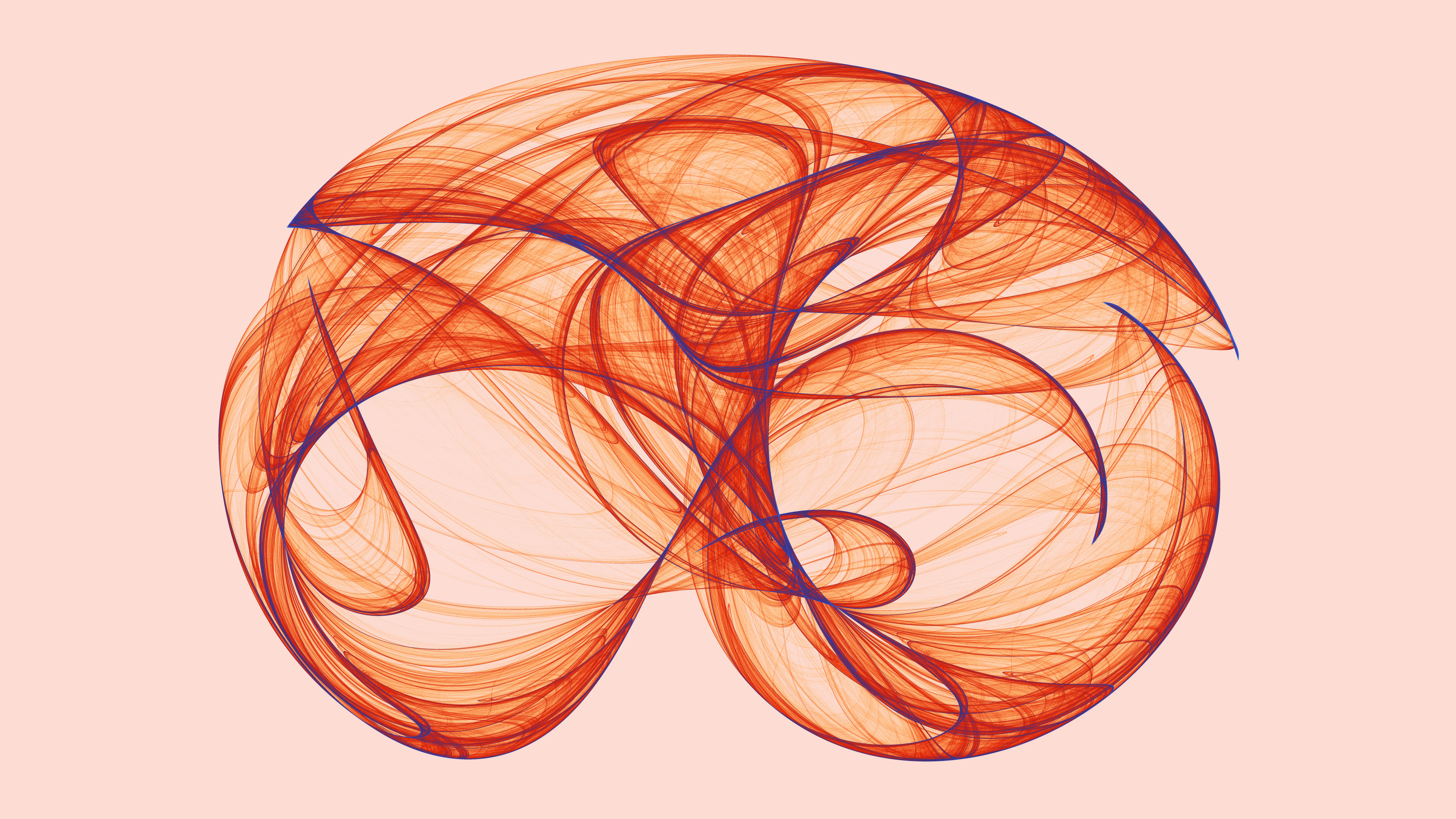{fig-align="center" width="465"}::: {style="font-family: Georgia; text-align: center; font-size: 17px"}**But how did our protagonists find themselves immersed in this captivating world of chaos and beauty?**:::It all began one rainy afternoon, as they stumbled upon an old book tucked away in the dusty corner of a library. Its pages whispered tales of strange attractors, chaotic systems that defied predictability yet exuded a haunting allure. Intrigued, our protagonist embarked on a journey of exploration, armed with nothing but curiosity and a genuine desire to unravel the mysteries of chaos.## What Are Strange Attractors?In math, a dynamical system tells us how a point in space changes over time using some fancy functions. An attractor is like a magnetic force that pulls points toward certain values over time, no matter where they start from. Simple attractors are kind of like fixed points or loops that the system settles into. But things get interesting with strange attractors. They're like wild, unpredictable whirlpools in math space where the system can roam around without repeating itself.One of the most famous strange attractors, discovered by this person named [Kiyohiro Ikeda](https://scholar.google.co.jp/citations?user=91qO-ocAAAAJ&hl=ja), is named after him. It's all described by these equations:$$x_{n+1}= 1+u(x_n \cos t_n −y_n \sin t_n)$$$$y_{n+1} = u (x_n \sin t_n + y_n \cos t_n)$$with $u ≥ 0.6$ and$$t_n = 0.4 − \dfrac{6}{1+ x_n^2 + y^2_n}$$In this example, our *imaginary* point moves in a 2D-dimensional space, since we just need `(x, y)` coordinates to describe its movement. In the previous system, time is represented by `n`. As you can see, Ikeda’s system only depends on one parameter, called `u`. The location of the point at `n` depends only on its location at `n-1`. For example, this image shows the trajectories of $2000$ random points following this previous equation with $u=0.918$:```{r, eval=FALSE}u=0.918 #Parameter between 0 and 1n=2000 #Number of particlesm=40 #Number of iterationsikeda=data.frame(it=1,x1=runif(n, min = -40, max = 40), y1=runif(n, min = -40, max = 40))ikeda$x2=1+u*(ikeda$x1*cos(0.4-6/(1+ikeda$x1^2+ikeda$y1^2))-ikeda$y1*sin(0.4-6/(1+ikeda$x1^2+ikeda$y1^2)))ikeda$y2= u*(ikeda$x1*sin(0.4-6/(1+ikeda$x1^2+ikeda$y1^2))+ikeda$y1*cos(0.4-6/(1+ikeda$x1^2+ikeda$y1^2)))for (k in 1:m){df=as.data.frame(cbind(rep(k+1,n),ikeda[ikeda$it==k,]$x2,ikeda[ikeda$it==k,]$y2,1+u*(ikeda[ikeda$it==k,]$x2*cos(0.4-6/(1+ikeda[ikeda$it==k,]$x2^2+ikeda[ikeda$it==k,]$y2^2))-ikeda[ikeda$it==k,]$y2*sin(0.4-6/(1+ikeda[ikeda$it==k,]$x2^2+ikeda[ikeda$it==k,]$y2^2))),u*(ikeda[ikeda$it==k,]$x2*sin(0.4-6/(1+ikeda[ikeda$it==k,]$x2^2+ikeda[ikeda$it==k,]$y2^2))+ikeda[ikeda$it==k,]$y2*cos(0.4-6/(1+ikeda[ikeda$it==k,]$x2^2+ikeda[ikeda$it==k,]$y2^2)))))names(df)=names(ikeda)ikeda=rbind(df, ikeda)}plot.new()par(mai = rep(0, 4), bg = "gray12")plot(c(0,0),type="n", xlim=c(-35, 35), ylim=c(-35,35))apply(ikeda, 1, function(x) lines(x=c(x[2],x[4]), y=c(x[3],x[5]), col = paste("gray", as.character(min(round(jitter(x[1]*80/(m-1)+(20*m-100)/(m-1), amount=5)), 100)), sep = ""), lwd=0.1))```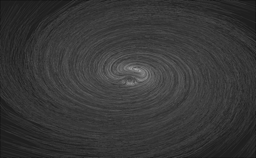{fig-align="center" width="549"}All points, regardless of their starting place, tend to end following the same path, represented in bright white colour. Another interesting property of strange attractors is that points that are very close at some instant, can differ significantly in the next step. This is why strange attractors are also known as *chaotic attractors*.## **Clifford Attractor's Mathematical Construction**Understanding the Clifford attractor was no easy feat. Its equations danced on the edge of complexity, teasing our protagonist with their elusive secrets. As they delved deeper into its mathematical underpinnings, our protagonist discovered a world of recursive equations and chaotic trajectories. The Clifford attractor, named after its creator [Clifford A. Pickover](https://en.wikipedia.org/wiki/Clifford_A._Pickover), was no ordinary mathematical construct. It was a window into the unpredictable nature of dynamical systems, where order emerged from chaos in the most unexpected ways. Now, we will experiment with Clifford attractors, but before diving into the experiment first we'll introduce this attractor formally.### **Formalism**A [Clifford Attractor](http://paulbourke.net/fractals/clifford) is a strange attractor defined by two iterative equations that determine the $x,y$ locations of discrete steps in the path of a particle across a 2D space, given a starting point $(x_0,y_0)$ and the values of four parameters $(a,b,c,d)$:$$x_{n+1} = \sin (ay_n) + c \cos (ax_n)$$$$y_{n+1} = \sin(b x_n) +d \cos(by_n)$$At each time step, the equations define the location for the following time step, and the accumulated locations show the areas of the 2D plane most commonly visited by the imaginary particle.# Unlocking Efficiency## Populating AttractorsThe Clifford attractor is a mathematical concept that falls under the broader category of Strange Attractors. It's a type of chaotic dynamical system that exhibits complex and beautiful patterns when iterated through a set of equations. The computational approach to exploring the Clifford attractor involves implementing these equations in code to visualize the attractor's behaviour.## **The Power of Iteration in Programming**Iteration lies at the heart of every programming language, serving as an indispensable technique for crafting robust, speedy, and concise code. It's the art of repeating tasks over and over, streamlining complex operations into manageable sequences. At its core lies the humble loop, a programming construct that condenses numerous lines of code into a compact, efficient form. By mastering iteration, programmers gain the ability to tackle daunting tasks with ease. With each loop iteration, they chip away at computational challenges, forging elegant solutions that are both powerful and succinct. Whether it's processing vast datasets or executing intricate algorithms, iteration empowers programmers to navigate complexity with finesse.In the realm of software development, efficiency is key. Writing efficient loops not only optimizes performance but also enhances code readability and maintainability. It allows developers to express their logic concisely, making it easier for others to understand and modify the code in the future. Indeed, the significance of iteration extends far beyond mere repetition. It embodies the essence of problem-solving in programming, enabling developers to transform abstract concepts into tangible solutions. As programmers harness the power of iteration, they unlock new realms of possibility, paving the way for innovation and discovery in the ever-evolving landscape of technology.# **Strange Attractors: An R Experiment**## **Recursivity & Creative Coding**Learning to code can be quite hard. Apart from the difficulties of learning a new *language*, following a book can be quite boring. One of the best ways to become a good programmer is to choose *small and funny* experiments oriented to training specific techniques of programming. In this tutorial, we will learn to combine C++ with R to create efficient loops. We will also learn interesting things about `ggplot2`, a very important package for data visualization. The *excuse* to do all this is to create beautiful images using a mathematical concept called *Strange Attractors*, which we will discuss briefly also. Combining art and coding is often called *generative art*, so be ready because after following this tutorial you can discover a new use of R to fall for as I am. Here we go!In R, you can do this using the `for()` function. For example, this loop calculates the mean of each column of a data frame called `df()` :```{r,message=FALSE,warning=FALSE}library(tidyverse)n <- 1000 # Rows of data frame# df with 4 columns and n rows sampled from N(0,1)df <- tibble( a = rnorm(n), b = rnorm(n), c = rnorm(n), d = rnorm(n))output <- vector("double", ncol(df)) # Empty output# For loopfor (i in 1:ncol(df)) { output[[i]] <- mean(df[[i]])}output```In the previous example, we repeated 4 times the task (which is the *piece* of code inside the curly brackets). Another way to do iterations in R, sometimes more efficient than a `for` loop, is by using the *apply* family. This is how the previous loop can be rewritten using the `apply()` function:```{r,eval=FALSE}output <- apply(df, 2, mean)output```These approaches have limitations. For example, if you want to use the result of an iteration as the input of the next one, you can not use *apply*. Another one is that sometimes R is not enough fast, which makes the `for` function quite inefficient. When you face this kind of situation, a good option is combining C++ and R.To represent the trajectory of a particular point, we need to store in a data frame its locations at every single (discrete) moment. For example, this is how we can do it using a `for` loop:```{r,message=FALSE,warning=FALSE}# Parameters settinga <- -1.25b <- -1.25c <- -1.82d <- -1.91# Number of jumpsn <- 5# Initialization of df to store locations of pointdf <- data.frame(x = double(n+1), y = double(n+1))# The point starts at (0,0)df[1, "x"] <- 0df[1, "y"] <- 0# For loop to store locationsfor (i in 1:n) { df[i+1, "x"] <- sin(a*df[i, "y"])+c*cos(a*df[i, "x"]) df[i+1, "y"] <- sin(b*df[i, "x"])+d*cos(b*df[i, "y"])}df```As you can see, our point started at $(0,0)$ and jumped $5$ times (the number of jumps is represented by $n$). You can try to change $n$ from $5$ to $10000000$ and see what happens (disclaimer: be patient). A better approach to do it is using `purrr`, a functional programming package which provides useful tools for iterating through lists and vectors, generalizing code and removing programming redundancies. The `purrr` tools work in combination with functions, lists and vectors and results in code that is consistent and concise. This can be a `purrr` approach to our problem:```{r,message=FALSE,warning=FALSE}library(purrrlyr)n <- 5# Initialization of our data framedf <- tibble(x = numeric(n+1), y = numeric(n+1))# Convert our data frame into a listby_row(df, function(v) list(v)[[1L]], .collate = "list")$.out -> df# This function computes current location depending of previous onef <- function(j, k, a, b, c, d) { tibble( x = sin(a*j$y)+c*cos(a*j$x), y = sin(b*j$x)+d*cos(b*j$y) )}# We apply accumulate on our list to store all steps and convert into a data frameaccumulate(df, f, a, b, c, d) %>% map_df(~ .x) -> dfdf```Even this approach is not efficient since the `accumulate()` function must be applied on an existing object (the `df()` in our case)## **Combining C++ and R**The paragraph below extracted from Hadley Wickham’s [Advanced R](#0), explains the motivations of combining C++ and R:`Rcpp` makes it very simple to connect C++ to R and provides a clean, approachable API that lets you write high-performance code, insulated from R’s complex C API. Typical bottlenecks that C++ can address include:- Loops that can’t be easily vectorised because subsequent iterations depend on previous ones.- Recursive functions, or problems which involve calling functions millions of times. The overhead of calling a function in C++ is much lower than in R.- Problems that require advanced data structures and algorithms that R doesn’t provide. Through the standard template library (STL), C++ has efficient implementations of many important data structures, from ordered maps to double-ended queues.This code populates our data frame using C++:```{r,eval=FALSE}# Load in libarieslibrary(Rcpp)library(tidyverse)# Here comes the C++ codecppFunction('DataFrame createTrajectory(int n, double x0, double y0, double a, double b, double c, double d) { // create the columns NumericVector x(n); NumericVector y(n); x[0]=x0; y[0]=y0; for(int i = 1; i < n; ++i) { x[i] = sin(a*y[i-1])+c*cos(a*x[i-1]); y[i] = sin(b*x[i-1])+d*cos(b*y[i-1]); } // return a new data frame return DataFrame::create(_["x"]= x, _["y"]= y); } ')a <- -1.25b <- -1.25c <- -1.82d <- -1.91# Call the function starting at (0,0) to store 10M jumpsdf <- createTrajectory(10000000, 0, 0, a, b, c, d)head(df)```Note that, apart from `Rcpp`, we also loaded the tidyverse package. This is because we will use some of its features, as `dplyr` or `ggplot2`, later.The function `createTrajectory()` is written in `C++` and stores the itinerary of an initial point. You can try it to see that It’s extremely fast. In the previous example, I populated on the fly our data frame with 10 million points starting at $(0,0)$ in less than 5 seconds in a conventional laptop.## **Rendering the Plot with `ggplot()`**Once we have built our data frame, it’s time to represent it with `ggplot()`. Making graphics is a necessary skill and for this `ggplot()` is an amazing tool, which by the way, I encourage you to learn. Usually, a good visualization is the best way to show your results. R is an extraordinary tool for visualizing data and one of the most important libraries to do it is `ggplot2`: it is powerful, flexible and is updated to include functionalities regularly. Although its syntax may seem a bit strange at first, here are four important concepts from my point of view to help you out with understanding it:- It’s truly important to have clear the type of graph you want to plot: for each one there’s a different *geometry*: `geom_point` to represent points, `geom_line` to represent time series, `geom_bar` to do bar chars … Have a look to `ggplot2` package, there are many other types.- Each of those geometries needs to define what data is to be used and how. For example, as you will see in our graph, we placed on the x-axis the `x` column of our data frame `df` and `y` on the y-axis, so we did `aes(x = x, y = y)`.- You can also combine geometries. We didn’t do that for our example but you may want, for example, to combine bars and lines on the same plot. To do it you can just use `+` operator. This operator is very important: it doesn’t only combine geometries, it’s also used to add features to the plot as we did to define its aspect ratio (with `coord_equal`) or its appearance (with `theme_void`).- You can modify every detail of the look and feel of your graph but be patient. To begin with, I recommend the use of predefined themes as I did with `theme_void`. There are many of them and it’s is a *quick and easy* way to change the appearance of your plot: just a way of making life easier and simpler.The `ggplot2` package is a new world by itself and takes part of the `tidyverse`, a collection of efficient libraries designed to analyze data in a consistent way. This is how we can represent the points of our data frame:```{r,eval=FALSE,message=FALSE,warning=FALSE}ggplot(df, aes(x = x, y = y)) + geom_point(shape = 46, alpha = .01) + coord_equal() + theme_void() -> plotggsave("strange1.png", plot, height = 5, width = 5, units = 'in')```{fig-align="center" width="394"}Another Approach to write the code:```{r,eval=FALSE,message=FALSE,warning=FALSE}library(Rcpp)library(ggplot2)library(dplyr)opt = theme(legend.position = "none", panel.background = element_rect(fill="white"), axis.ticks = element_blank(), panel.grid = element_blank(), axis.title = element_blank(), axis.text = element_blank())cppFunction('DataFrame createTrajectory(int n, double x0, double y0, double a, double b, double c, double d) { // create the columns NumericVector x(n); NumericVector y(n); x[0]=x0; y[0]=y0; for(int i = 1; i < n; ++i) { x[i] = sin(a*y[i-1])+c*cos(a*x[i-1]); y[i] = sin(b*x[i-1])+d*cos(b*y[i-1]); } // return a new data frame return DataFrame::create(_["x"]= x, _["y"]= y); } ')a=-1.24458046630025b=-1.25191834103316 c=-1.81590817030519 d=-1.90866735205054df=createTrajectory(10000000, 0, 0, a, b, c, d)png("Clifford.png", units="px", width=1600, height=1600, res=300)ggplot(df, aes(x, y)) + geom_point(color="black", shape=46, alpha=.01) + optdev.off()```particularly using Rcpp to incorporate `C++` code within `R`, lies in its efficiency and versatility:1. **Efficiency**: By leveraging `C++` through `Rcpp`, computationally intensive tasks can be executed much faster compared to pure `R` code. `C++` is known for its performance, making it ideal for handling large data sets or complex calculations.2. **Versatility**: Integrating `C++` code within `R` expands the capabilities of the `R` language. It allows developers to access `C++` libraries and functionalities, enabling them to implement advanced algorithms or optimize existing code for better performance.3. **Ease of Use**: Despite the complexity of `C++`, `Rcpp` simplifies the process of incorporating `C++` code within `R` scripts. Developers can write `C++` functions directly within their `R` environment, avoiding the need for separate compilation and linking processes.4. **Interoperability**: The resulting code is seamlessly integrated with `R`, allowing users to interact with `C++` functions just like any other `R` function. This interoperability facilitates collaboration and code reuse within the R ecosystem.5. **Graphics and Visualization**: The code snippet demonstrates the seamless integration of `C++` computations with R's powerful visualization capabilities, particularly with `ggplot2`. This combination enables users to analyze and visualize data efficiently, enhancing the interpretability of results.6. **Scalability**: With `C++` optimization, code performance scales efficiently with increasing dataset sizes. This scalability is crucial for handling large-scale data analysis tasks commonly encountered in research, industry, and data science applications.The syntax of our plot is quite simple. Just two comments about it:- Shape is set to $46$, the smallest filled point. More info about shapes, [here](http://sape.inf.usi.ch/quick-reference/ggplot2/shape)- Since there are a lot of points, I make them transparent with alpha to take advantage on its overlapping and reveal patterns of shadows.## Playing with ParametersStrange attractors are extremely sensitive to their parameters. This feature makes them very entertaining as well as an infinite source of surprises. This is what happens to Clifford attractor when setting `a`, `b`, `c` and `d` parameters to `-1.2`, `-1.9`, `1.8` and `-1.6` respectively:```{r,eval=FALSE,message=FALSE,warning=FALSE}a <- -1.2b <- -1.9c <- 1.8d <- -1.6df <- createTrajectory(10000000, 0, 0, a, b, c, d)ggplot(df, aes(x = x, y = y)) + geom_point(shape = 46, alpha = .01) + coord_equal() + theme_void() -> plotggsave("strange2.png", plot, height = 5, width = 5, units = 'in')```{fig-align="center" width="363"}::: {style="font-family: Georgia; text-align: center; font-size: 17px"}***Don’t you feel like playing with parameters? From my point of view, this is a very classy way of spending your time.***:::## The General 2D-MapOnce we know what strange attractors *look like*, let’s try another family of them. This is the new formula we will experiment with:$$x_{n+1} = a_1+a_2x_n+a_3y_n+a_4 |x_n|^{a_5} +a_6|y_n|^{a_7}$$$$y_{n+1} = a_8 +a_9x_n +a_{10}y_n+a_{11}|x_n|^{a_{12}}+a_{13}|y_n|^{a_{14}}$$These attractors are localized mostly to a small region of the XY plane with *tentacles* that stretch out to large distances. If any of the exponents are negative and the attractor intersects the line along which the respective variable is zero, a point on the line maps to infinity. However, large values are visited infrequently by the orbit, so many iterations are required to determine that the orbit is unbounded. For this reason most of the attractors in the figures have holes in their interiors where their orbits are precluded from coming too close to their origins.```{r,eval=FALSE,message=FALSE,warning=FALSE}cppFunction('DataFrame createTrajectory(int n, double x0, double y0, double a1, double a2, double a3, double a4, double a5, double a6, double a7, double a8, double a9, double a10, double a11, double a12, double a13, double a14) { // create the columns NumericVector x(n); NumericVector y(n); x[0]=x0; y[0]=y0; for(int i = 1; i < n; ++i) { x[i] = a1+a2*x[i-1]+ a3*y[i-1]+ a4*pow(fabs(x[i-1]), a5)+ a6*pow(fabs(y[i-1]), a7); y[i] = a8+a9*x[i-1]+ a10*y[i-1]+ a11*pow(fabs(x[i-1]), a12)+ a13*pow(fabs(y[i-1]), a14); } // return a new data frame return DataFrame::create(_["x"]= x, _["y"]= y); } ')a1 <- -0.8a2 <- 0.4a3 <- -1.1a4 <- 0.5a5 <- -0.6a6 <- -0.1a7 <- -0.5a8 <- 0.8a9 <- 1.0a10 <- -0.3a11 <- -0.6a12 <- -0.3a13 <- -1.2a14 <- -0.3df <- createTrajectory(10000000, 1, 1, a1, a2, a3, a4, a5, a6, a7, a8, a9, a10, a11, a12, a13, a14)ggplot(df) + geom_point(aes(x = x, y = y), shape = 46, alpha = .01, color = "black") + coord_fixed() + theme_void() -> plotggsave("strange3.png", plot, height = 5, width = 5, units = 'in')mx <- quantile(df$x, probs = 0.05)Mx <- quantile(df$x, probs = 0.95)my <- quantile(df$y, probs = 0.05)My <- quantile(df$y, probs = 0.95)df %>% filter(x > mx, x < Mx, y > my, y < My) -> dfggplot(df) + geom_point(aes(x = x, y = y), shape = 46, alpha = .01, color = "black") + coord_fixed() + theme_void() -> plotggsave("strange3.png", plot, height = 5, width = 5, units = 'in')```{fig-align="center" width="344"}Sometimes you will need to process the data frame after you generate it since:- Extreme values can hide the pattern as happened before or even *scape* to infinite (solution: remove outliers).- Some images can be quite *boring*: from my point of view, the more *distributed* ae points on the XY plane, the nicer is the resulting image (solution: try with a small data frame and keep it if some measure of dispersion over the plane or the individual axis is high enough; in this case, compute the big picture).To conclude, let’s change the appearance of our plot. We will use the `theme` function to customize it setting the background color to black and adding a white line as frame.```{r,eval=FALSE,warning=FALSE,message=FALSE}opt <- theme(legend.position = "none", panel.background = element_rect(fill="black", color="white"), plot.background = element_rect(fill="black"), axis.ticks = element_blank(), panel.grid = element_blank(), axis.title = element_blank(), axis.text = element_blank())plot <- ggplot(df) + geom_point(aes(x = x, y = y), shape = 46, alpha = .01, color = "white") + coord_fixed() + optggsave("strange4.png", plot, height = 5, width = 5, units = 'in')```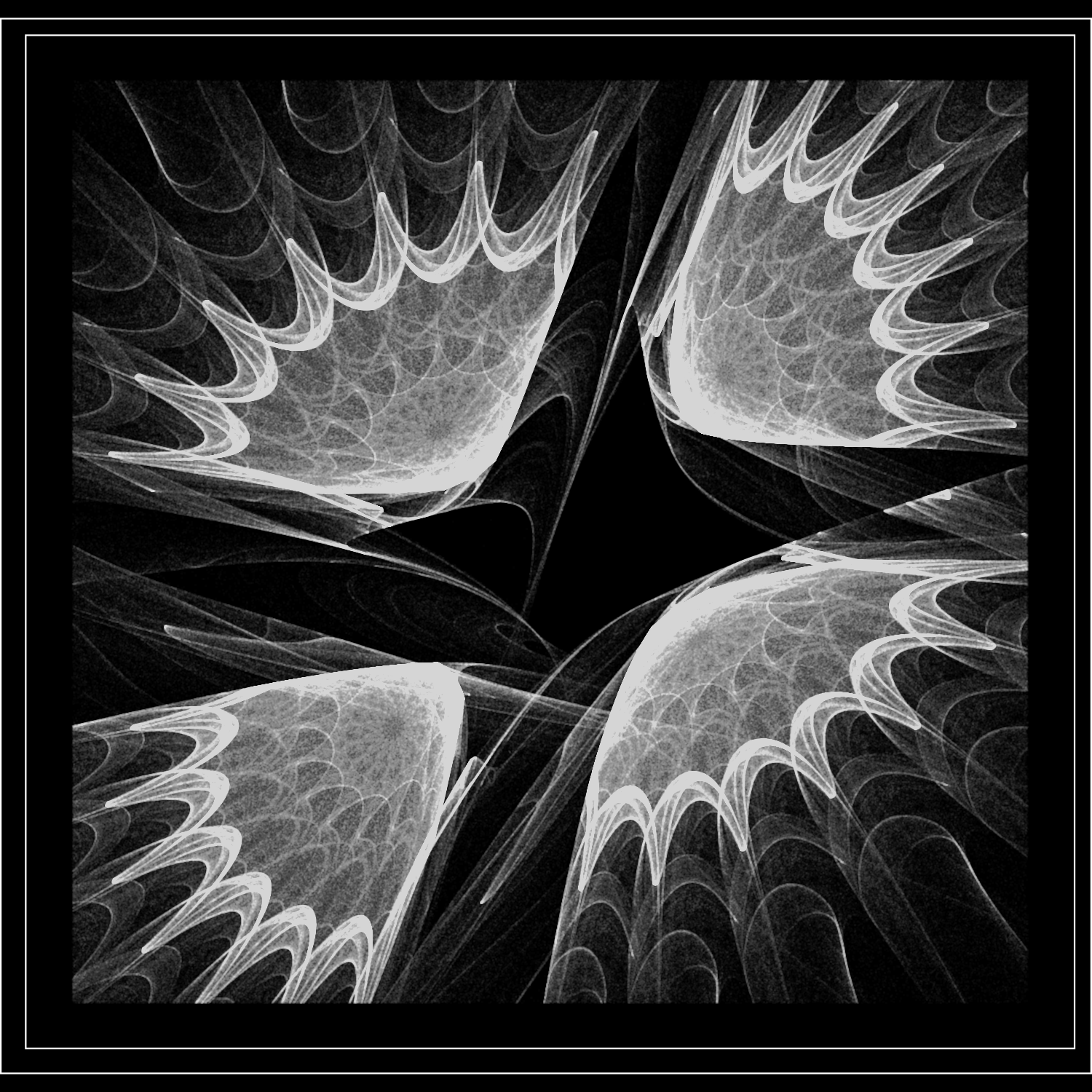{fig-align="center" width="347"}This code snippet is a demonstration of using the *Clifford attractor* and the *DeJong attractor* to generate and visualize complex patterns.```{r,eval=FALSE,message=FALSE,warning=FALSE}library("compiler")mapxy <- function(x, y, xmin, xmax, ymin=xmin, ymax=xmax) { sx <- (width - 1) / (xmax - xmin) sy <- (height - 1) / (ymax - ymin) row0 <- round( sx * (x - xmin) ) col0 <- round( sy * (y - ymin) ) col0 * height + row0 + 1}dejong <- function(x, y) { nidxs <- length(mat) counts <- integer(length=nidxs) for (i in 1:npoints) { xt <- sin(a * y) - cos(b * x) y <- sin(c * x) - cos(d * y) x <- xt idxs <- mapxy(x, y, -2, 2) counts <- counts + tabulate(idxs, nbins=nidxs) } mat <<- mat + counts}clifford <- function(x, y) { ac <- abs(c)+1 ad <- abs(d)+1 nidxs <- length(mat) counts <- integer(length=nidxs) for (i in 1:npoints) { xt <- sin(a * y) + c * cos(a * x) y <- sin(b * x) + d * cos(b * y) x <- xt idxs <- mapxy(x, y, -ac, ac, -ad, ad) counts <- counts + tabulate(idxs, nbins=nidxs) } mat <<- mat + counts}#color vectorcvec <- grey(seq(0, 1, length=10))#can also try other colours, see help(rainbow)#cvec <- heat.colors(10)#we end up with npoints * n pointsnpoints <- 8n <- 100000 width <- 600height <- 600#make some random pointsrsamp <- matrix(runif(n * 2, min=-2, max=2), nr=n)#compile the functionssetCompilerOptions(suppressAll=TRUE)mapxy <- cmpfun(mapxy)dejong <- cmpfun(dejong)clifford <- cmpfun(clifford)#dejonga <- 1.4b <- -2.3c <- 2.4d <- -2.1mat <- matrix(0, nr=height, nc=width)dejong(rsamp[,1], rsamp[,2])#this applies some smoothing of low valued points, from A.N. Spiess#QUANT <- quantile(mat, 0.5)#mat[mat <= QUANT] <- 0dens <- log(mat + 1)/log(max(mat))par(mar=c(0, 0, 0, 0))image(t(dens), col=cvec, useRaster=T, xaxt='n', yaxt='n')#clifforda <- -1.4b <- 1.6c <- 1.0d <- 0.7mat <- matrix(0, nr=height, nc=width)#QUANT <- quantile(mat, 0.5)#mat[mat <= QUANT] <- 0clifford(rsamp[,1], rsamp[,2])dens <- log(mat + 1)/log(max(mat))par(mar=c(0, 0, 0, 0))image(t(dens), col=cvec, useRaster=T, xaxt='n', yaxt='n')```::: {layout-ncol="2"}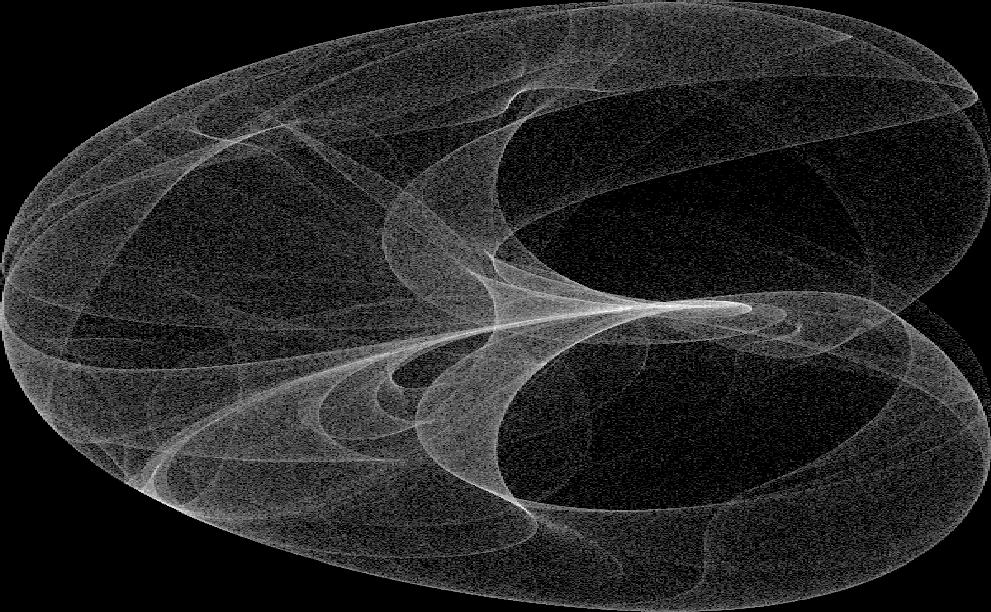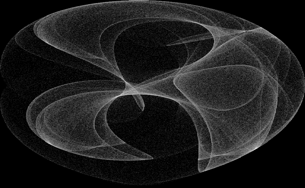:::Let's break down the code and provide a justification for each part:1. **Function Definitions**: - **`mapxy`**: Imagine you have a grid like a chessboard, and you want to find the position of a specific square on that grid. This function helps map any point (x, y) on a continuous plane to a specific position on a grid by considering the boundaries of the grid. - **`dejong`**: Think of this as a magical equation that takes a point (x, y) and transforms it into another point based on certain rules. Each iteration of this equation generates a new point, creating a trail of points over time. - **`clifford`**: Similar to **`dejong`**, this equation also transforms points, but in a different way. It has its own set of rules that create a distinct pattern when applied iteratively.2. **Color Vector Definition**: - **`cvec`**: Think of this as a palette of colors. Just like an artist selects colors for their painting, we're selecting grayscale colors here to represent different intensities of the patterns we'll generate.3. **Parameters and Settings**: - **`npoints`**, **`n`**, **`width`**, **`height`**: These parameters control the characteristics of our final image. For example, **`npoints`** determines how many points we'll generate for each attractor, and **`width`** and **`height`** specify the dimensions of our image. - **`rsamp`**: This matrix contains random points scattered within a specific range. These points serve as starting positions for our attractor patterns.4. **Function Compilation**: - **`setCompilerOptions`** and **`cmpfun`**: Imagine you're preparing a recipe. Compiling these functions is like preparing ingredients in advance so that when it's time to cook (run the functions), everything is ready and runs smoothly.5. **Attractor Generation**: - **`dejong`** and **`clifford`**: Here, we're actually running the "magic equations" defined earlier on our random points (**`rsamp`**). These equations generate attractor patterns by transforming each point iteratively. - Optional smoothing: We can apply a smoothing technique to our generated patterns to make them look nicer. This technique removes noise or low-valued points from our pattern, enhancing its visual appeal.6. **Visualization**: - **`image`**: Finally, we visualize our attractor patterns using the **`image`** function. It's like projecting our patterns onto a screen. The color vector (**`cvec`**) helps represent different intensities in the patterns, creating a visually appealing image. - Plotting parameters adjustment: We tweak some settings to remove unnecessary labels and margins from our plot, ensuring a clean and focused display of our attractor patterns.This code snippet efficiently generates and visualizes complex attractor patterns using the DeJong and Clifford attractor functions. It demonstrates the power of iteration in programming to create intricate and visually stunning results. Additionally, function compilation enhances performance, making it suitable for handling large datasets and generating high-resolution images.# **Conclusion**But the journey was far from over. As our protagonist navigated the twists and turns of the Clifford attractor, they realized that its true beauty lay not in its predictability, but in its boundless creativity. With each iteration, they discovered new patterns, new symmetries, and new wonders that left them in awe of the chaotic dance unfolding before them.# **Further Reading****More about recursivity and `ggplot`:**- Hadley’s [R for Data Science](https://r4ds.had.co.nz/iteration.html) and [Advanced R](https://adv-r.hadley.nz/rcpp.html): the first one covers iteration methods (including functional ones) as well as `ggplot` and the second one introduces `Rcpp` to use C++ when R is not fast enough.**More about strange attractors:**- [Strange Attractors: Creating Patterns in Chaos](http://sprott.physics.wisc.edu/sa.htm), by Julien C. Sprott: a beautiful book which describes a big amount of different attractors including equations and examples of their patterns.# **References**K.Ikeda, Multiple-valued Stationary State and its Instability of the Transmitted Light by a Ring Cavity System, Opt. Commun. 30 257-261 (1979); K. Ikeda, H. Daido and O. Akimoto, Optical Turbulence: Chaotic Behavior of Transmitted Light from a Ring Cavity, Phys. Rev. Lett. 45, 709–712 (1980){fig-align="center" width="389"}


