Comprehensive Guide to Numerical Integration and ODEs in R
Mastering deSolve, odeintr, and More for Complex ODE Integration
R Progaming
Mathematics
Author
Abhirup Moitra
Published
June 12, 2024
Solving Stiff Differential Equations
deSolve() Package
Description: The deSolve package is a comprehensive tool for solving differential equations in R. It is capable of handling a variety of differential equations, including ordinary differential equations (ODEs), partial differential equations (PDEs), and delay differential equations (DDEs). The package includes several solvers designed for stiff systems, such as lsoda, lsode, lsodes, vode, and daspk.
Example:
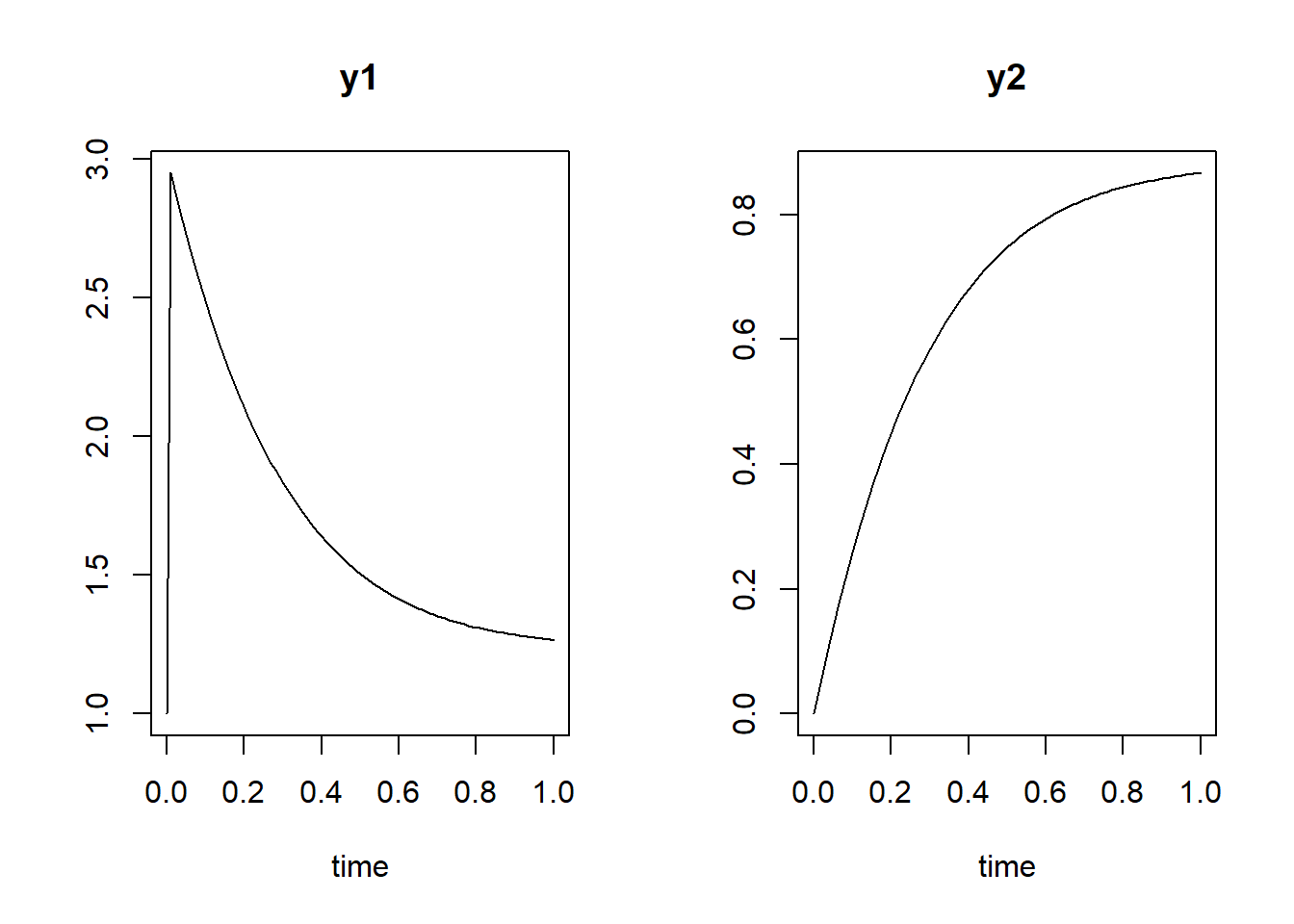
library(deSolve)# Define the stiff ODE functionstiffODE <-function(t, y, parms) { dy1 <--1000* y[1] +3000-2000* y[2] dy2 <- y[1] - y[2] -0.5* y[2]^3list(c(dy1, dy2))}# Initial state and parametersstate <-c(y1 =1, y2 =0)times <-seq(0, 1, by =0.01)# Solve the stiff ODE using lsoda solverout <-ode(y = state, times = times, func = stiffODE, parms =NULL, method ="lsoda")plot(out)
odeintr() Package
Description: The odeintr package is designed for integrating differential equations in R, utilizing the Boost.odeint package as its integration engine. This package offers several notable features, including simple specification of the ODE system and named, dynamically settable system parameters. It provides intelligent defaults, which are easily overridden, and supports a wide range of integration methods for compiled systems through various stepper types.
One of the standout features of odeintr is its fully automated compilation of ODE systems specified in C++. It also supports simple OpenMP vectorization for large systems, although this feature is currently broken in the latest Boost release. Results from integrations are returned as a straightforward data frame, ready for analysis and plotting.
The package allows users to specify custom observers in R, which can return arbitrary data. There are three options for calling the observer: at regular intervals, after each update step, or at specified times. Users can also alter the system state and restart simulations from where they left off. Additionally, odeintr can compile an implicit solver with symbolic evaluation of the Jacobian, and it provides the ability to save and edit the generated C++ code easily.
#installation #install.packages(odeintr) # released# Install and load the packagedevtools::install_github("thk686/odeintr", force =TRUE)
Using GitHub PAT from the git credential store.
Downloading GitHub repo thk686/odeintr@HEAD
── R CMD build ─────────────────────────────────────────────────────────────────
* checking for file 'C:\Users\maths\AppData\Local\Temp\Rtmpm41qZK\remotes1a2046713a2a\thk686-odeintr-1f1e7f9/DESCRIPTION' ... OK
* preparing 'odeintr':
* checking DESCRIPTION meta-information ... OK
* cleaning src
* checking for LF line-endings in source and make files and shell scripts
* checking for empty or unneeded directories
* building 'odeintr_1.7.1.tar.gz'
Warning: file 'odeintr/configure' did not have execute permissions: corrected
Installing package into 'C:/Users/maths/AppData/Local/R/win-library/4.3'
(as 'lib' is unspecified)
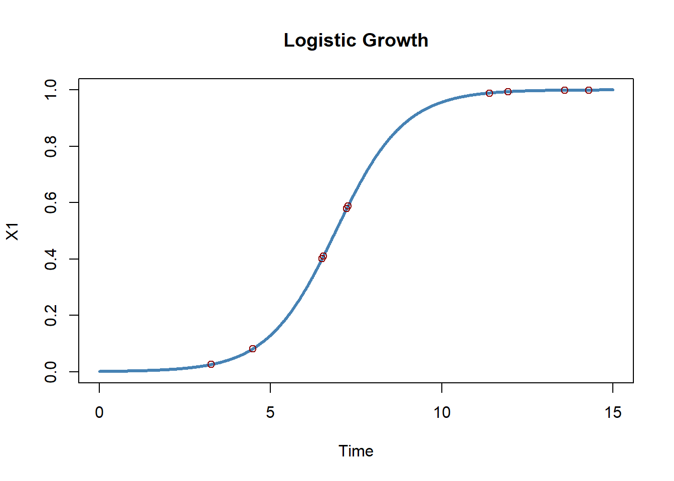
library(odeintr)# Define the ODE functiondxdt =function(x, t) x * (1- x)# Integrate the systemsystem.time({ x =integrate_sys(dxdt, 0.001, 15, 0.01)})
   user  system elapsed
   0.02    0.00    0.02
# Plot the resultsplot(x, type ="l", lwd =3, col ="steelblue", main ="Logistic Growth")# Compile the systemcompile_sys("logistic", "dxdt = x * (1 - x)")# Integrate the compiled systemsystem.time({ x =logistic(0.001, 15, 0.01)})
   user  system elapsed
      0       0       0
# Plot the results of the compiled systemplot(x, type ="l", lwd =3, col ="steelblue", main ="Logistic Growth")points(logistic_at(0.001, sort(runif(10, 0, 15)), 0.01), col ="darkred")
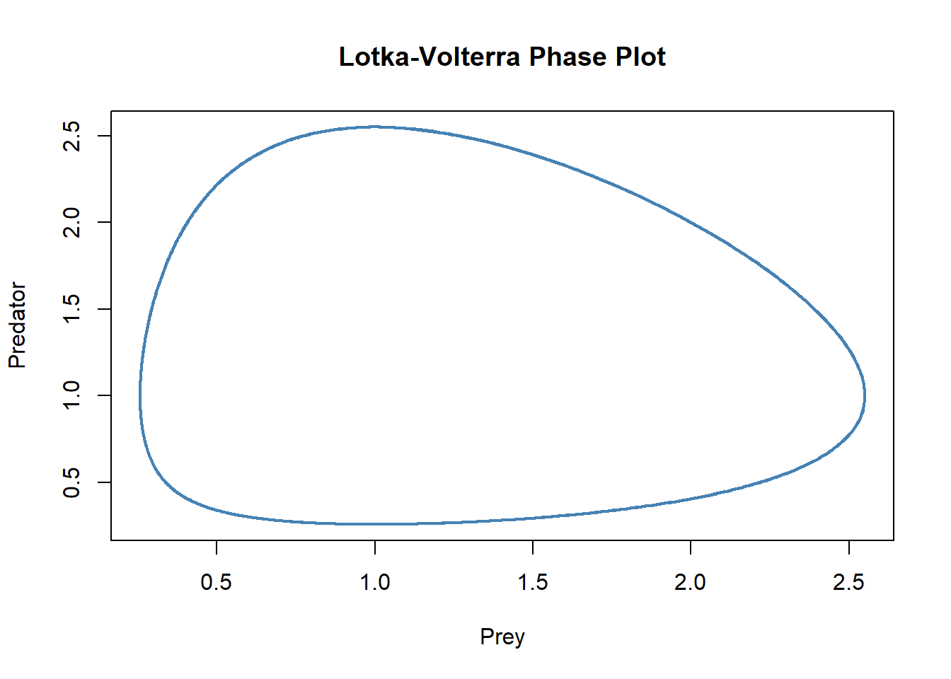
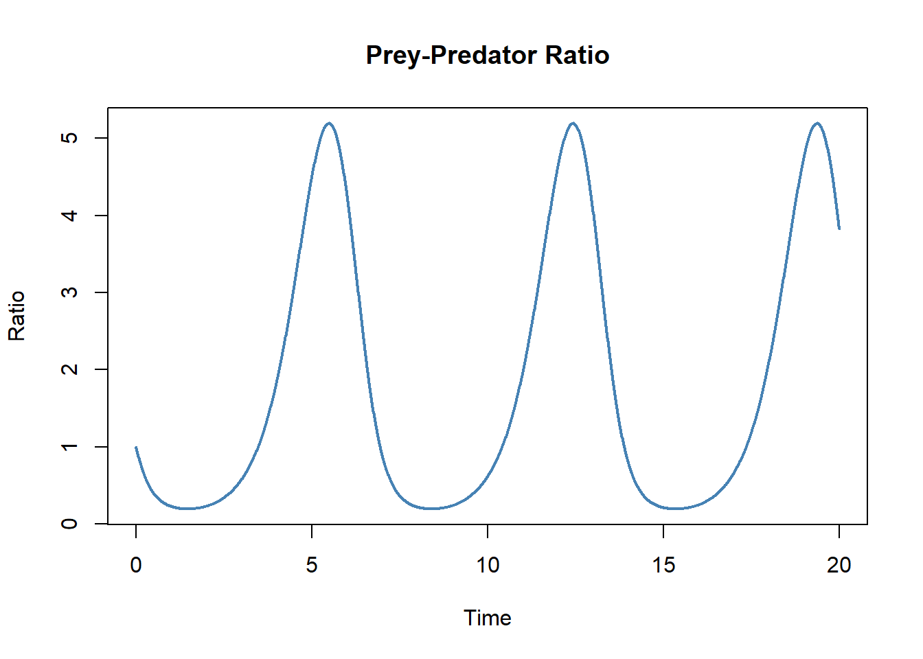
compile_implicit("stiff", Stiff.sys)x =stiff(c(2, 1), 5, 0.001)plot(x[, 1:2], type ="l", lwd =2, col ="steelblue")lines(x[, c(1, 3)], lwd =2, col ="darkred")
Numerical Integration
pracma() Package
Description: The pracma package offers a wide range of numerical methods, including tools for numerical integration. It is useful for performing one-dimensional integration as well as handling more complex mathematical tasks.
library(pracma)
Attaching package: 'pracma'
The following object is masked from 'package:deSolve':

    rk4
# Define the function to integratef <-function(x) sin(x)# Perform numerical integrationresult <-integral(f, 0, pi)print(result)
[1] 2
cubature() Package
Description: The cubature package is designed for adaptive multivariate integration over hypercubes. It is particularly useful for higher-dimensional integration problems and can handle a variety of complex integrals efficiently.
library(cubature)# Define the multivariate function to integratef <-function(x) x[1]^2+ x[2]^2# Perform numerical integration over [0, 1] x [0, 1]result <-adaptIntegrate(f, lowerLimit =c(0, 0), upperLimit =c(1, 1))print(result$integral)
[1] 0.6666667
Base R integrate Function
Description: The integrate function in base R is a straightforward tool for performing numerical integration of one-dimensional functions. It is easy to use and provides reliable results for a wide range of integrals.
# Define the function to integratef <-function(x) x^2# Perform numerical integrationresult <-integrate(f, 0, 1)print(result$value)
[1] 0.3333333
These notes should provide your readers with a clear understanding of the recommended packages for solving stiff differential equations and performing numerical integration in R, along with example codes and references for further reading.
R has several packages that are well-regarded for integrating and solving differential equations. Here are some of the most popular ones:
deSolve():
This package provides functions to solve initial value problems of differential equations, including ordinary differential equations (ODEs), partial differential equations (PDEs), and delay differential equations (DDEs).
It supports both stiff and non-stiff systems and offers a variety of solvers.
Example usage
library(deSolve)# Define the ODE functionmodel <-function(time, state, parameters) {with(as.list(c(state, parameters)), { dN <- r * Nreturn(list(c(dN))) })}# Initial state and parametersstate <-c(N =1)parameters <-c(r =0.1)times <-seq(0, 100, by =1)# Solve the ODEout <-ode(y = state, times = times, func = model, parms = parameters)
PBSddesolve():
This package is designed for solving delay differential equations (DDEs) and ordinary differential equations (ODEs). It is useful if your system involves delays.
Example usage
library(PBSddesolve)
-----------------------------------------------------------
PBSddesolve 1.13.4 -- Copyright (C) 2007-2024 Fisheries and Oceans Canada
(based on solv95 by Simon Wood)

A complete user guide 'PBSddesolve-UG.pdf' is located at
C:/Users/maths/AppData/Local/R/win-library/4.3/PBSddesolve/doc/PBSddesolve-UG.pdf

Demos include 'blowflies', 'cooling', 'icecream', and 'lorenz'
They can be run two ways:

1. Using 'utils' package 'demo' function, run command
> demo(icecream, package='PBSddesolve', ask=FALSE)

2. Using package 'PBSmodelling', run commands
> require(PBSmodelling); runDemos()
and choose PBSddesolve and then one of the four demos.

Packaged on 2024-01-04
Pacific Biological Station, Nanaimo

All available PBS packages can be found at
https://github.com/pbs-software
-----------------------------------------------------------
# Define the DDE functionmodel <-function(t, y, parms) { dy <- parms["r"] * y[1]return(list(dy))}# Initial state and parametersstate <-c(N =1)parameters <-c(r =0.1)times <-seq(0, 100, by =1)# Solve the DDEout <-dde(y = state, times = times, func = model, parms = parameters)
ReacTran():
Useful for solving reaction-transport equations, especially in one, two, or three dimensions. It builds on the deSolve package.
Example usage
library(ReacTran)
Loading required package: rootSolve
Attaching package: 'rootSolve'
The following objects are masked from 'package:pracma':

    gradient, hessian
Loading required package: shape
library(deSolve)# Example setup for ReacTran
Solving integral equations in R can be accomplished using several packages, each with its specific strengths for different types of integral equations. Here are a few notable ones:
pracma():
This package provides numerical tools for a variety of mathematical operations, including solving integral equations.
Example usage
library(pracma)# Define the integral equationf <-function(x) x^2# Solve the integral from 0 to 1result <-integral(f, 0, 1)print(result)
[1] 0.3333333
DEoptim:
This package is primarily used for optimization, but it can also handle integral equations through its optimization routines by minimizing the difference between the left and right sides of the integral equation.
Example usage:
library(DEoptim)
Loading required package: parallel
DEoptim package
Differential Evolution algorithm in R
Authors: D. Ardia, K. Mullen, B. Peterson and J. Ulrich
# Define the integral equationf <-function(x) x^2integral_eq <-function(a) abs(integral(f, 0, a) - target_value)# Use DEoptim to solve for atarget_value <-1result <-DEoptim(integral_eq, lower =0, upper =2)
The integrate function in base R can be used to perform numerical integration, which is essential for solving certain integral equations.
Example usage
f <-function(x) x^2# Solve the integral from 0 to 1result <-integrate(f, 0, 1)print(result$value)
[1] 0.3333333
Cubature:
This package is used for adaptive multivariate integration over hypercubes, which can be useful for higher-dimensional integral equations.
Example usage
library(cubature)# Define the multivariate integral functionf <-function(x) x[1]^2+ x[2]^2# Solve the integral over [0, 1] x [0, 1]result <-adaptIntegrate(f, lowerLimit =c(0, 0), upperLimit =c(1, 1))print(result$integral)
[1] 0.6666667
integral (pracma):
In addition to the general pracma package, the specific integral function can be quite handy.
Example usage
library(pracma)# Define the integral equation functionf <-function(x) sin(x)# Perform the integration over the range 0 to piresult <-integral(f, 0, pi)print(result)
[1] 2
Each of these packages can handle different types of integral equations, and their selection depends on the specific problem and complexity of the equations you are dealing with. For many general purposes, the integrate function in base R and the pracma package’s integral function are very effective and straightforward to use.