Most of you will have heard about the number called the golden ratio. It appears, for example, in the book/film The da Vinci Code and in many articles, books, and school projects, which aim to show how mathematics is important in the real world. It has been described by many authors (including the writer of the da Vinci Code) as the basis of all of the beautiful patterns in nature and it is sometimes referred to as the divine proportion. It is claimed that much of art and architecture contains features in proportions given by the golden ratio. Since the time of the ancient Greeks artists, designers, thinkers, scientists, and engineers, have been fascinated by the golden ratio also denoted \(\phi\). The golden ratio has over the centuries even been considered the perfect illustration of beauty.
Before going to introduce how to execute the golden spiral programming code I’m going to share small code chunks which will help you to understand how Fibonacci numbers usually generate.
One of the interesting properties of the Fibonacci sequence is the ratio of each pair of adjacent terms in the sequence. When dividing the nth term in the sequence by the n-1 term in the sequence, the ratio converges to approximately 1.618034 as the value for n increases. This value is the Golden Ratio (or Golden Mean).
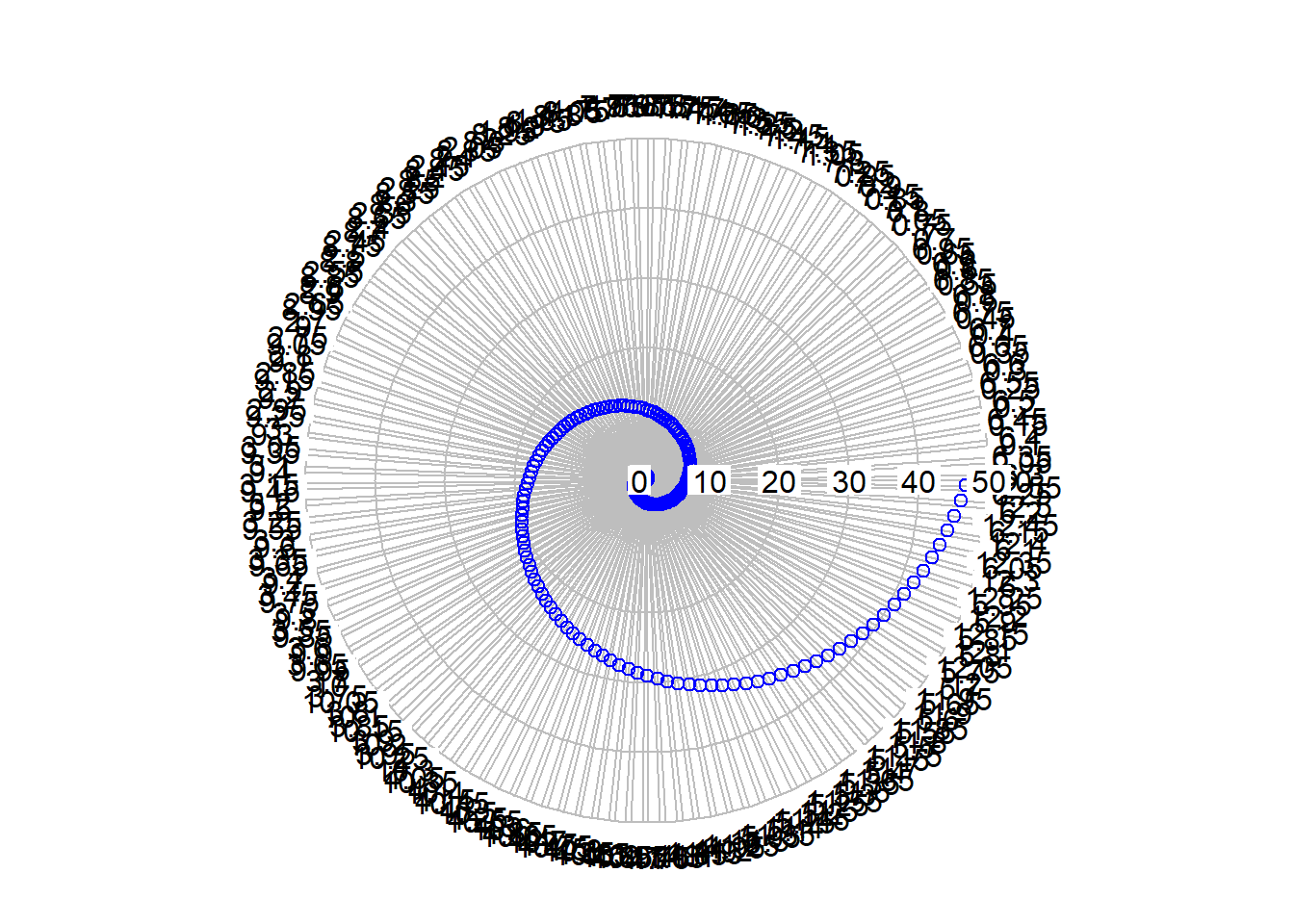
In polar coordinates, this special instance of a logarithmic spiral’s functional representation can be simplified to \(r(t)= e^{0.30635t}\). For every quarter turn, the corresponding point on the spiral is a factor of phi further from the origin (r is this distance), with phi the golden ratio - the same one obtained from dividing any 2 sufficiently big successive numbers on a Fibonacci sequence, which is how the golden ratio, the golden spiral, and Fibonacci sequences are linked concepts.
Let’s do 2 full circles. First create a sequence of angle values theta. Since \(2\pi\) is the equivalent of a circle in polar coordinates, we need to have distances from the origin for values between 0 and \(4\pi\).
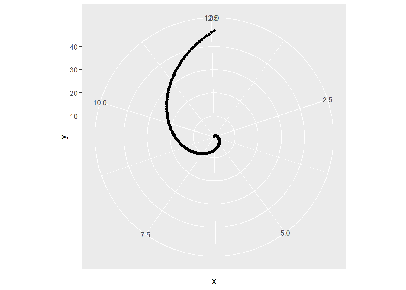
Plotting the function using coord_polar in ggplot2 does not work as intended. Unexpectedly, the x-axis keeps extending instead of circling back once a full circle is reached. Turns out coord_polar might not be intended to plot elements in polar vector format.
Code
ggplot(data.frame(x = seq_theta, y = dist_from_origin), aes(x,y)) +geom_point() +coord_polar(theta="x")
With that established and the original objective of the exercise achieved, it still would be nice to be able to accomplish this using ggplot2. To do so, the created sequence above needs to be converted to cartesian coordinates. The rectangular function equivalent of the golden spiral function r(t) defined above is \(a(t) = (r(t) cos(t), r(t) sin(t))\). It’s not too hard to come up with a hack to convert one to the other.
cartesian_golden_spiral <-function(theta) { a <-polar_golden_spiral(theta)*cos(theta) b <-polar_golden_spiral(theta)*sin(theta)c(a,b)}
Applying that function to the same series of angles from above and stitching the resulting coordinates in a data frame. Note I’m enclosing the first expression in brackets, which prints it immediately, which is useful when the script is run interactively.
---title: "Programming and Visulization Golden Spiral"author: "Abhirup Moitra"date: 2023-02-15format: html: code-fold: true code-tools: trueeditor: visualcategories : [Mathematics, R Programming]image: spiral.jpg---# **Golden Spiral**Most of you will have heard about the number called the golden ratio. It appears, for example, in the book/film [The da Vinci Code](https://en.wikipedia.org/wiki/The_Da_Vinci_Code_(film)) and in many articles, books, and school projects, which aim to show how mathematics is important in the real world. It has been described by many authors (including the writer of the da Vinci Code) as the basis of all of the beautiful patterns in nature and it is sometimes referred to as the divine proportion. It is claimed that much of art and architecture contains features in proportions given by the golden ratio. Since the time of the ancient Greeks artists, designers, thinkers, scientists, and engineers, have been fascinated by the golden ratio also denoted $\phi$. The golden ratio has over the centuries even been considered the perfect illustration of beauty.Before going to introduce how to execute the golden spiral programming code I'm going to share small code chunks which will help you to understand how Fibonacci numbers usually generate.```{r,eval=FALSE,message=FALSE,warning=FALSE}#install.packages(c("UsingR","numbers"))library(UsingR)library(numbers)n<-40s <- seq(1:n)fib <- as.integer(sapply(s, fibonacci)) fib#View(fib)x1<- ifelse(seq(1:n)%%2 ==1, fib, 0)y1<- ifelse(seq(1:n)%%2 ==0, fib, 0)x2 <-ifelse(seq(1:n)%%4==1, x1,-x1)y2 <-ifelse(seq(1:n)%%4==2, y1,-y1)x <- ifelse(x2 >0, log(x2), ifelse(x2<0, -log(-x2),0))y <- ifelse(y2 >0, log(y2), ifelse(y2<0, -log(-y2),0))plot(x,y)lines(x,y, col="blue")```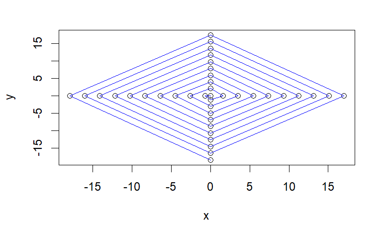{fig-align="center" width="527"}## **Property**One of the interesting properties of the Fibonacci sequence is the ratio of each pair of adjacent terms in the sequence. When dividing the nth term in the sequence by the n-1 term in the sequence, the ratio converges to approximately 1.618034 as the value for n increases. This value is the Golden Ratio (or Golden Mean).```{r,eval=FALSE,message=FALSE,warning=FALSE}GoldenRatio=(1+sqrt(5))/2i=3fib=c(1,1)while(abs(fib[i-1]/fib[i-2]-GoldenRatio)>0.001){ fib[i] <- fib[i-1]+fib[i-2] i=i+1}print(fib)fib=c(1,1)ratio <- c()for (i in 3:20) { ratio <- c(ratio, fib[i-1]/fib[i-2]) fib[i] <- fib[i-1]+fib[i-2] i=i+1}plot(ratio, pch=19,col='red')lines(ratio, pch=19,col='red')abline(h=GoldenRatio, col='blue')legend('topright', legend=c('f(i)/f(i+1)', 'GoldenRatio'), col=c('red', 'blue'), lwd=2)```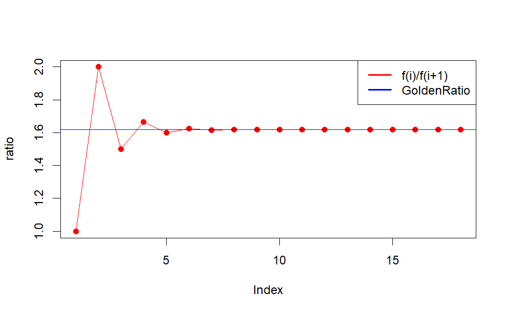{fig-align="center" width="584"}## **Import Libraries**```{r,message=FALSE}#install.packages(c("tidyverse","plotrix"))library(tidyverse)library(plotrix)```## **Transforming into Polar Coordinates**In polar coordinates, this special instance of a logarithmic spiral's functional representation can be simplified to $r(t)= e^{0.30635t}$. For every quarter turn, the corresponding point on the spiral is a factor of phi further from the origin (r is this distance), with phi the golden ratio - the same one obtained from dividing any 2 sufficiently big successive numbers on a Fibonacci sequence, which is how the golden ratio, the golden spiral, and Fibonacci sequences are linked concepts.```{r,message=FALSE}polar_golden_spiral <- function(theta) exp(0.30635*theta)```Let's do 2 full circles. First create a sequence of angle values theta. Since $2\pi$ is the equivalent of a circle in polar coordinates, we need to have distances from the origin for values between 0 and $4\pi$.```{r,message=FALSE}seq_theta <- seq(0,4*pi,by=0.05)dist_from_origin <- sapply(seq_theta,polar_golden_spiral)```Plotting the function using **coord_polar** in ggplot2 does not work as intended. Unexpectedly, the x-axis keeps extending instead of circling back once a full circle is reached. Turns out **coord_polar** might not be intended to plot elements in polar vector format.```{r,message=FALSE}ggplot(data.frame(x = seq_theta, y = dist_from_origin), aes(x,y)) + geom_point() + coord_polar(theta="x")```With that established and the original objective of the exercise achieved, it still would be nice to be able to accomplish this using ggplot2. To do so, the created sequence above needs to be converted to cartesian coordinates. The rectangular function equivalent of the golden spiral function r(t) defined above is $a(t) = (r(t) cos(t), r(t) sin(t))$. It's not too hard to come up with a hack to convert one to the other.```{r,message=FALSE}plotrix::radial.plot(dist_from_origin, seq_theta,rp.type="s", point.col = "blue")``````{r,eval=FALSE,message=FALSE}cartesian_golden_spiral <- function(theta) { a <- polar_golden_spiral(theta)*cos(theta) b <- polar_golden_spiral(theta)*sin(theta) c(a,b)}```Applying that function to the same series of angles from above and stitching the resulting coordinates in a data frame. Note I'm enclosing the first expression in brackets, which prints it immediately, which is useful when the script is run interactively.```{r,eval=FALSE,message=FALSE,results='hide',warning=FALSE}(serie <- sapply(seq_theta,cartesian_golden_spiral))df <- data.frame(t(serie))```## Final Result:With everything now ready in the right coordinate system, it's now only a matter of setting some options to make the output look acceptable.```{r,eval=FALSE,message=FALSE}ggplot(df, aes(x=X1,y=X2)) + geom_path(color="blue") + theme(panel.grid.minor = element_blank(), axis.text.x = element_blank(), axis.text.y = element_blank()) + scale_y_continuous(breaks = seq(-20,20,by=10)) + scale_x_continuous(breaks = seq(-20,50,by=10)) + coord_fixed() + labs(title = "Golden spiral", subtitle = "Another view on the Fibonacci sequence", caption = "www.linkedin.com/in/abhirup-moitra-7a66731a6 https://github.com/ABHI20-STAT.", x = "", y = "")```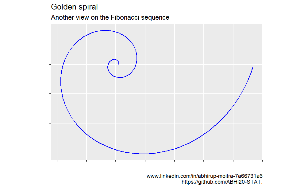{fig-align="center" width="603"}## References:1. <https://www.mathsisfun.com/numbers/fibonacci-sequence.html>2. <https://www.livescience.com/37470-fibonacci-sequence.html>3. <https://www.geeksforgeeks.org/python-plotting-fibonacci-spiral-fractal-using-turtle/>