Code
x <- 15
xThe topic of calculus is fundamentally about mathematical functions and the operations that are performed on them. The concept of “mathematical function” is an idea. If we are going to use a computer language to work with mathematical functions, we will need to translate them into some entity in the computer language. That is, we need a language construct to represent functions and the quantities functions take as input and produce as output.
If you happen to have a background in programming, you may well be thinking that the choice of representation is obvious. For quantities, use numbers. For functions, use R-language functions. That is indeed what we are going to do, but as you’ll see, the situation is just a little more complicated than that. A little, but that little complexity needs to be dealt with from the beginning.
In this session we are going implement the operations of calculus along with related operations such as graphing and solving.
The complexity mentioned in the previous section stems the uses and real-world situations to which we want to be able to apply the mathematical idea of functions. The inputs taken by functions and the outputs produced by them are not necessarily numbers. Often, they are quantities. Consider these examples of quantities: money, speed, blood pressure, height, volume. Isn’t each of these quantities a number? Not quite. Consider money. We can count, add, and subtract money – just like we count, add, and subtract with numbers. But money has an additional property: the kind of currency. Money as an idea is an abstraction of the kind sometimes called a dimension. Other dimensions are length, time, volume, temperature, area, angle, luminosity, bank interest rate, and so on. When we are dealing with a quantity that has dimension, it’s not enough to give a number to say “how much” of that dimension we have. We need also to give units. Many of these are familiar in everyday life. For instance, the dimension of length is quantified with units of meters, or inches, or miles, or parsecs, and so on. The dimension of money is measured with euros, dollars, renminbi, and so on. Area as a dimension is quantified with square-meters, or square-feet, or hectares, or acres, etc.
Unfortunately, most mathematics texts treat dimension and units by ignoring them. This leads to confusion and error when an attempt is made to apply mathematical ideas to quantities in the real world. Here we will be using functions and calculus to work with real-world quantities. We can’t afford to ignore dimension and units. Unfortunately, mainstream computer languages like R and Python and JavaScript do not provide a systematic way to deal with dimension and units automatically. In R, for example, we can easily write
x <- 15
xwhich stores a quantity under the name x. But the language bawks at something like
y <- 12 meters
Error: unexpected symbol in "y <- 12 meters"
Lacking a proper computer notation for representing dimensioned quantities with their units, we need some other way to keep track of things.
This style of using the name of a quantity as a reminder of the dimension and units of the quantity is outside the tradition of mathematical notation. In high-school math, you encountered \(x\) and \(y\) and \(y\) and \(\theta\) You might even have seen subscripts used to be more specific, for instance \(x_0\) Someone trained in physics will know the traditional and typical uses of letters. \(x\) is likely a position, \(t\) is likely a time, and \(x_0\) is the position at time zero.
For experts working extensively with algebraic manipulations, this elaborate system of nomenclature may be unavoidable and even optimal. But when the experts are implementing their ideas as computer programs, they have to use a much more mundane approach to naming things: character strings like Reynolds.
There can be an advantage to the mundane approach. In this session, we’ll be working with calculus, which is used in a host of fields. We’re going to be drawing examples from many fields. And so we want our quantities to have names that are easy to recognize and remember. Things like income and blood_pressure and farm_area. If we tried to stick to x and y and z, our computer notation would become incomprehensible to the human reader and thus easily subject to error.
R, like most computer languages, has a programming construct to represent operations that take one or more inputs and produce an output. In R, these are called “functions.” In R, everything you do involves a function, either explicitly or implicitly.
Let’s look at the R version of a mathematical function, exponentiation. The function is named exp and we can look at the programming it contains
exp## function (x) .Primitive("exp")Not much there, except computer notation. In R, functions can be created with the key word function. For instance, to create a function that translates yearly income to daily income, we could write
as_daily_income <- function(yearly_income) {
  yearly_income / 365
}
The name selected for the function, as_daily_income, is arbitrary. We could have named the function anything at all. (It’s a good practice to give functions names that are easy to read and write and remind you what they are about.) After the keyword function, there is a pair of parentheses. Inside the parentheses are the names being given to the inputs to the function. There’s just one input to as_daily_income which we called yearly_income just to help remind us what the function is intended to do. But we could have called the input anything at all. The part function(yearly_income) specifies that the thing being created will be a function and that we are calling the input yearly_income. After this part comes the body of the function. The body contains R expressions that specify the calculation to be done. In this case, the expression is very simple: divide yearly_income by 365 – the (approximate) number of days in a year. It’s helpful to distinguish between the value of an input and the role that the input will play in the function. A value of yearly income might be 61362 (in, say, dollars). To speak of the role that the input plays, we use the word argument. For instance, we might say something like, “as_yearly_income is a function that takes one argument.” Following the keyword function and the parentheses where the arguments are defined comes a pair of curly braces { and } containing some R statements. These statements are the body of the function and contain the instructions for the calculation that will turn the inputs into the output.
Here’s a surprising feature of computer languages like R … The name given to the argument doesn’t matter at all, so long as it is used consistently in the body of the function. So the programmer might have written the R function this way:
as_daily_income <- function(x) {
  x / 365
  }
or even,
as_daily_income <- function(ghskelw) {
  ghskelw / 365
}
All of these different versions of as_daily_income() will do exactly the same thing and be used in exactly the same way, regardless of the name given for the argument. Like this:
as_daily_income(70560)[1] 193.3151Often, functions have more than one argument. The names of the arguments are listed between the parentheses following the keyword function, like this:
as_daily_income <- function(yearly_income, duration) {
  yearly_income / duration
}
In such a case, to use the function we have to provide all the arguments. So, with the most recent two-argument definition of as_daily_income(), the following use generates an error message:
as_daily_income(70560)
## Error in as_daily_income(61362): argument "duration" is missing, with no default
Instead, specify both arguments:
as_daily_income <- function(yearly_income, duration) {
  yearly_income / duration
}
as_daily_income(61362, 365)
[1] 168.1151One more aspect of function arguments in R … Any argument can be given a default value. It’s easy to see how this works with an example:
as_daily_income <- function(yearly_income, duration = 365) {
  yearly_income / duration
}
With the default value for duration the function can be used with either one argument or two:
as_daily_income(99000,duration = 365)[1] 271.2329To close, let’s return to the exp function, which is built-in to R. The single argument to exp was named x and the body of the function is somewhat cryptic: .Primitive("exp").
It will often be the case that the functions we create will have bodies that don’t involve traditional mathematical expressions like \(x/d\). As you’ll see in later session, in the modern world many mathematical functions are too complicated to be represented by algebraic notation.
Don’t be put off by such non-algebra function bodies. Ultimately, what you need to know about a function in order to use it are just three things:
What are the arguments to the function and what do they stand for.
What kind of thing is being produced by the function.
That the function works as advertised, e.g. calculating what we would write algebraically as \(e^x\).
Recall that the names selected by the programmer of a function are arbitrary. You would use the function in exactly the same way even if the names were different. Similarly, when using the function you can pick yourself what expression will be the value of the argument.
For example, suppose you want to calculate \(100e^{−2.5}\).
100 * exp(-2.5)But it’s likely that the \(-2.5\) is meant to stand for something more general. For instance, perhaps you are calculating how much of a drug is still in the body ten days after a dose of 100 mg was administered. There will be three quantities involved in even a simple calculation of this: the dosage, the amount of time since the dose was taken, and what’s called the “time constant” for elimination of the drug via the liver or other mechanisms. (To follow this example, you don’t have to know what a time constant is. But if you’re interested, here’s an example. Suppose a drug has a time constant of 4 days. This means that a 63% of the drug will be eliminated during a 4-day period.)
In writing the calculation, it’s a good idea to be clear and explicit about the meaning of each quantity used in the calculation. So, instead of 100 * exp(-2.5), you might want to write:
dose <- 100 # mg
duration <- 10 # days
time_constant <- 4 # days
dose * exp(- duration / time_constant)
[1] 8.2085Even better, you could define a function that does the calculation for you:
drug_remaining <- function(dose, duration, time_constant) {
  dose * exp(- duration / time_constant)
}
Then, doing the calculation for the particular situation described above is a matter of using the function:
drug_remaining(dose = 100, duration = 10, time_constant = 4)By using good, descriptive names and explicitly labelling which argument is which, you produce a clear and literate documentation of what you are intending to do and how someone else, including “future you,” should change things for representing a new situation.
We’ve been using R functions to represent the calculation of quantities from inputs like the dose and time constant of a drug.
But R functions play a much bigger role than that. Functions are used for just about everything, from reading a file of data to drawing a graph to finding out what kind of computer is being used. Of particular interest to us here is the use of functions to represent and implement the operations of calculus. These operations have names that you might or might not be familiar with yet: differentiation, integration, etc.
When a calculus or similar mathematical operation is being undertaken, you usually have to specify which variable or variables the operation is being done “with respect to.” To illustrate, consider the conceptually simple operation of drawing a graph of a function. More specifically, let’s draw a graph of how much drug remains in the body as a function of time since the dose was given. The basic pharmaceutics of the process is encapsulated in the drug_remaining() function. So what we want to do is draw a graph of drug_remaining().
Recall that drug_remaining() has three arguments: dose, duration, and time_constant. The particular graph we are going to draw shows the drug remaining as a function of duration. That is, the operation of graphing will be with respect to duration. We’ll consider, say, a dose of 100 mg of a drug with a time constant of 4 days, looking perhaps at the duration interval from 0 days to 20 days.
In this session, we’ll be using operations provided by the mosaic and mosaicCalc packages for R. The operations from these packages have a very specific notation to express with respect to. That notation uses the tilde character, ~. Here’s how to draw the graph we want, using the package’s slice_plot() operation:
install.packages("mosaicCalc")
library(mosaicCalc)
slice_plot(
  drug_remaining(dose = 100, time_constant = 4, duration = t) ~ t,
  domain(t = 0:20))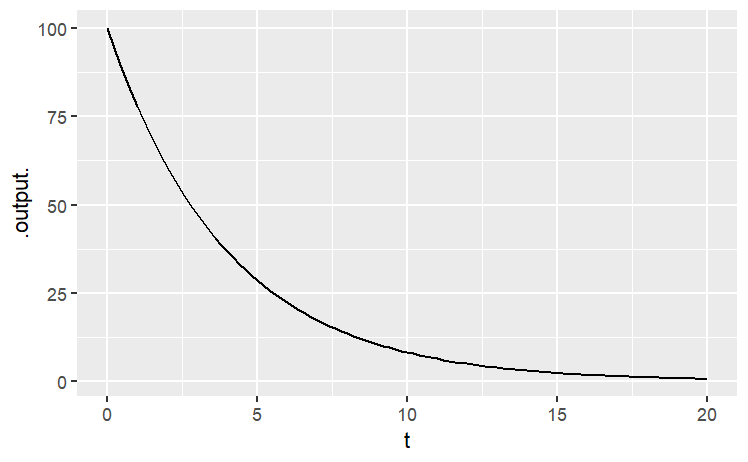
A proper graph would be properly labelled, for instance the horizontal axis with “Time (days)” and the vertical axis with “Remaining drug (mg)”. You’ll see how to do that in the next part, which explores the function-graphing operation in more detail.
In this lesson, you will learn how to use R to graph mathematical functions. It’s important to point out at the beginning that much of what you will be learning – much of what will be new to you here – actually has to do with the mathematical structure of functions and not R.
Recall that a function is a transformation from an input to an output. Functions are used to represent the relationship between quantities. In evaluating a function, you specify what the input will be and the function translates it into the output.
In much of the traditional mathematics notation you have used, functions have names like \(f\) or \(g\) or \(y\), and the input is notated as \(x\). Other letters are used to represent parameters. For instance, it’s common to write the equation of a line this way
\[ y= mx+c \]
In order to apply mathematical concepts to realistic settings in the world, it’s important to recognize three things that a notation like \(y=mx+c\) does not support well:
Real-world relationships generally involve more than two quantities. (For example, the Ideal Gas Law in chemistry, \(PV=nRT\), involves three variables: pressure, volume, and temperature.) For this reason, you will need a notation that lets you describe the multiple inputs to a function and which lets you keep track of which input is which.
Real-world quantities are not typically named \(x\) and \(y\), but are quantities like “cyclic AMP concentration” “membrane voltage” or “government expenditures”. Of course, you could call all such things \(x\) or \(y\), but it’s much easier to make sense of things when the names remind you of the quantity being represented.
Real-world situations involve many different relationships, and mathematical models of them can involve different approximations and representations of those relationships. Therefore, it’s important to be able to give names to relationships, so that you can keep track of the various things you are working with
For these reasons, the notation that you will use needs to be more general than the notation commonly used in high-school algebra. At first, this will seem odd, but the oddness doesn’t have to do so much with the fact that the notation is used by the computer so much as for the mathematical reasons given above.
But there is one aspect of the notation that stems directly from the use of the keyboard to communicate with the computer. In writing mathematical operations, you’ll use expressions like a * b and 2 ^ n and a / b rather than the traditional \(\frac{a}{b}\) or \(2^n\) or \(ab\), and you will use parentheses both for grouping expressions and for applying functions to their inputs.
In plotting a function, you need to specify several things:
What is the function. This is usually given by an expression, for instance m * x + b or A * x ^ 2 or sin(2 * t) Later on, you will also give names to functions and use those names in the expressions, much like sin is the name of a trigonometric function.
What are the inputs. Remember, there’s no reason to assume that \(x\) is always the input, and you’ll be using variables with names like G and cAMP. So you have to be explicit in saying what’s an input and what’s not. The R notation for this involves the ~ (“tilde”) symbol. For instance, to specify a linear function with \(x\) as the input, you can write m * x + b ~ x
What range of inputs to make the plot over. Think of this as the bounds of the horizontal axis over which you want to make the plot.
The values of any parameters. Remember, the notation m * x + b ~ x involves not just the variable input x but also two other quantities, m and b. To make a plot of the function, you need to pick specific values for m and b and tell the computer what these are.
There are three graphing functions in {mosaicCalc} that enable you to graph functions, and to layer those plots with graphs of other functions or data. These are:
slice_plot() for functions of one variable.
contour_plot() for functions of two variables.
interactive_plot() which produces an HTML widget for interacting with functions of two variables.
slice_plot(3 * x - 2 ~ x, domain(x = range(0, 10)))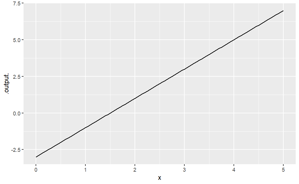
Often, it’s natural to write such relationships with the parameters represented by symbols. (This can help you remember which parameter is which, e.g., which is the slope and which is the intercept. When you do this, remember to give a specific numerical value for the parameters, like this:
m = -3
b = -2
slice_plot(m * x + b ~ x, domain(x = range(0, 10)))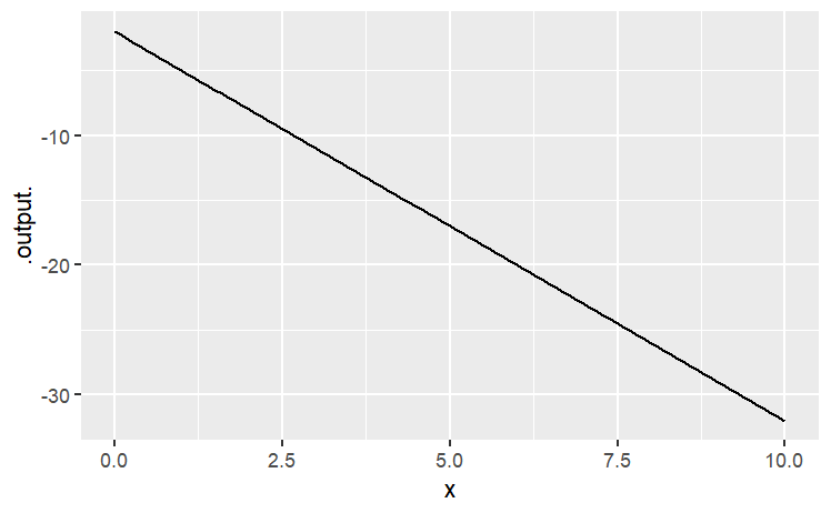
A = 100
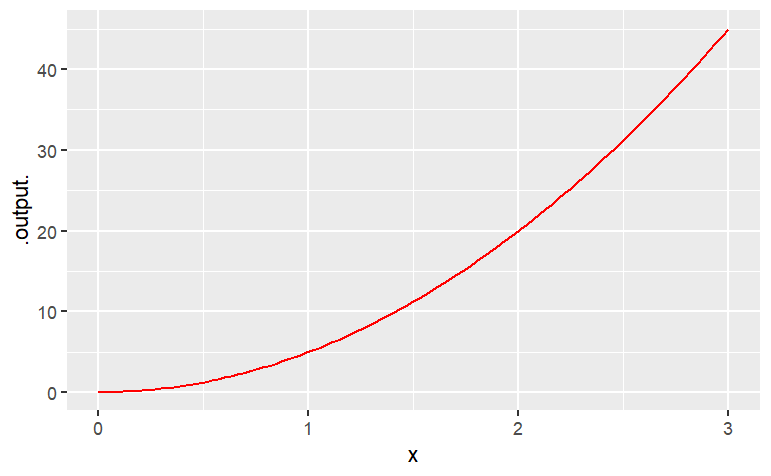
slice_plot( A * x ^ 2 ~ x, domain(x = range(-2, 3)))
A = 5
slice_plot( A * x ^ 2 ~ x, domain(x = range(0, 3)), color="red" )
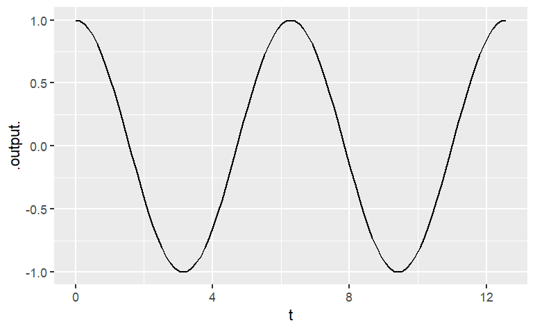
slice_plot( cos(t) ~ t, domain(t = range(0,4*pi) ))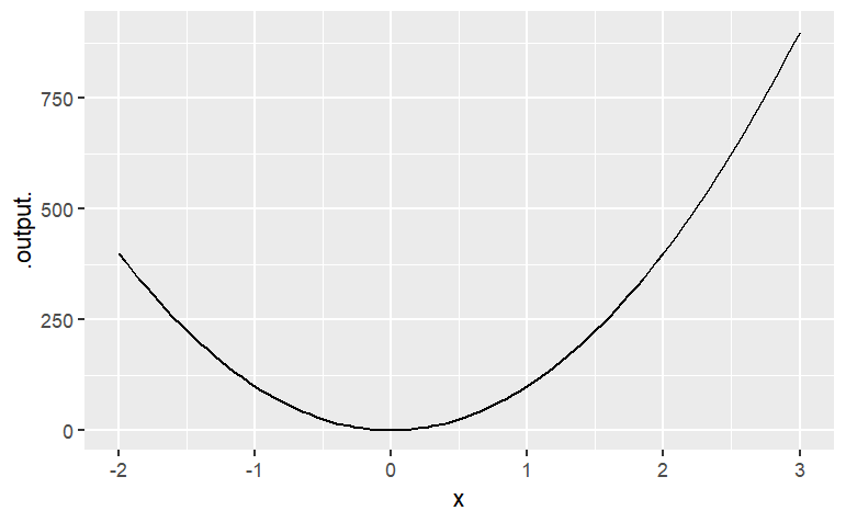
You can use makeFun( ) to give a name to the function. For instance:
g  <- makeFun(2*x^2 - 5*x + 2 ~ x)
slice_plot(g(x) ~ x , domain(x = range(-2, 2)))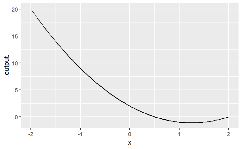
Once the function is named, you can evaluate it by giving an input. For instance:
g(x = 2)## [1] 0g(x = 5)[1] 27Of course, you can also construct new expressions from the function you have created. Try this somewhat complicated expression:
slice_plot(sqrt(abs(g(x))) ~ x, domain(x = range(-5,5)))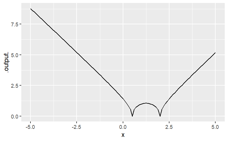
x <- 10
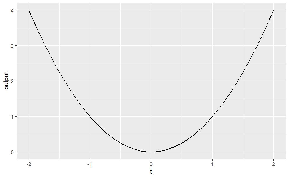
slice_plot(A * x ^ 2 ~ A, domain(A = range(-2, 3)))Explain why the graph doesn’t look like a parabola, even though it’s a graph of \(Ax^2\)
Translate each of these expressions in traditional math notation into a plot. Hand in the command that you gave to make the plot (not the plot itself).
\(4x−7\) in the window \(x\) from \(0\) to \(10\).
\(\cos5x\) in the window \(x\) from \(−1\) to \(1\).
\(\cos2t\) in the window \(t\) from \(0\) to \(5\).
\(\sqrt{t} \cos t\) in the window \(t\) from \(0\) to \(5.\)
Find the value of each of the functions above at \(x=10.543\) or at \(t=10.543\). (Hint: Give the function a name and compute the value using an expression like g(x = 10.543) or f(t = 10.543).
Pick the closest numerical value
\(32.721, 34.721, 35.172, 37.421, 37.721\)
\(-0.83, -0.77, -0.72, -0.68, 0.32, 0.42, 0.62\)
\(-0.83, -0.77, -0.72, -0.68, -0.62, 0.42, 0.62\)
\(-2.5, -1.5, -0.5, 0.5, 1.5, 2.5\)
Reproduce each of these plots. Hand in the command you used to make the identical plot:
Often, the mathematical models that you will create will be motivated by data. For a deep appreciation of the relationship between data and models, you will want to study statistical modeling. Here, though, we will take a first cut at the subject in the form of curve fitting, the process of setting parameters of a mathematical function to make the function a close representation of some data.
This means that you will have to learn something about how to access data in computer files, how data are stored, and how to visualize the data. Fortunately, R and the mosaic package make this straightforward.
The data files you will be using are stored as spreadsheets on the Internet. Typically, the spreadsheet will have multiple variables; each variable is stored as one column. (The rows are “cases,” sometimes called “data points.”) To read the data in to R, you need to know the name of the file and its location. Often, the location will be an address on the Internet.
Here, we’ll work with "Income-Housing.csv", which is located at "http://www.mosaic-web.org/go/datasets/Income-Housing.csv". This file gives information from a survey on housing conditions for people in different income brackets in the US. (Source: Susan E. Mayer (1997) What money can’t buy: Family income and children’s life chances Harvard Univ. Press p. 102.)
Here’s how to read it into R:
Housing = read.csv("http://www.mosaic-web.org/go/datasets/Income-Housing.csv")There are two important things to notice about the above statement. First, the read.csv() function is returning a value that is being stored in an object called housing. The choice of Housing as a name is arbitrary; you could have stored it as x or Equador or whatever. It’s convenient to pick names that help you remember what’s being stored where. Second, the name “http://www.mosaic-web.org/go/datasets/Income-Housing.csv” is surrounded by quotation marks. These are the single-character double quotes, that is, " and not repeated single quotes ' ' or the backquote ` . Whenever you are reading data from a file, the name of the file should be in such single-character double quotes. That way, R knows to treat the characters literally and not as the name of an object such ashousing`. Once the data are read in, you can look at the data just by typing the name of the object (without quotes!) that is holding the data. For instance,
view(Housing)All of the variables in the data set will be shown (although just four of them are printed here). You can see the names of all of the variables in a compact format with the names( ) command:
names(Housing)
Housing$Income
Housing$CrimeProblem
Even though the output from names( ) shows the variable names in quotation marks, you won’t use quotations around the variable names. Spelling and capitalization are important. If you make a mistake, no matter how trifling to a human reader, R will not figure out what you want. For instance, here’s a misspelling of a variable name, which results in nothing (NULL) being returned.
Housing$crimSometimes people like to look at datasets in a spreadsheet format, each entry in a little cell. In RStudio, you can do this by going to the “Workspace” tab and clicking the name of the variable you want to look at. This will produce a display like the following:
View(Housing)You probably won’t have much use for this, but occasionally it is helpful. Usually the most informative presentation of data is graphical. One of the most familiar graphical forms is the scatter-plot, a format in which each “case” or “data point” is plotted as a dot at the coordinate location given by two variables. For instance, here’s a scatter plot of the fraction of household that regard their neighborhood as having a crime problem, versus the median income in their bracket.
gf_point(CrimeProblem ~ Income, data = Housing )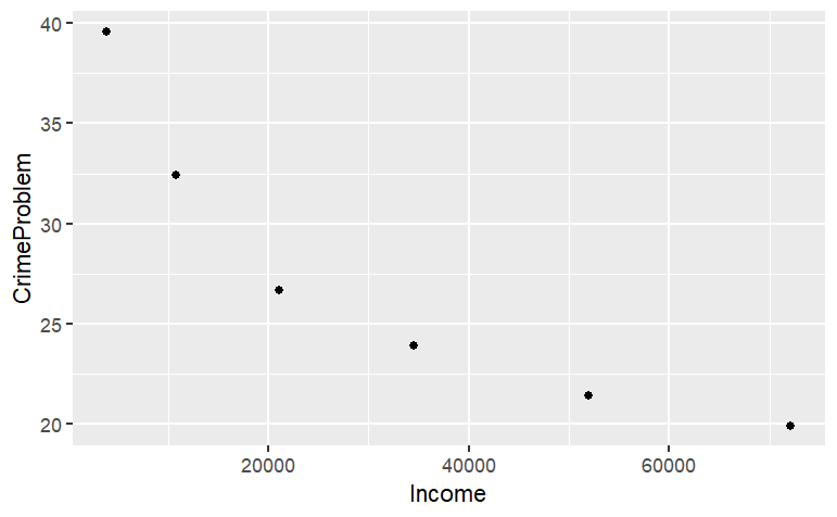
The R statement closely follows the English equivalent: “plot as points CrimeProblem versus (or, as a function of) Income, using the data from the housing object.
Graphics are constructed in layers. If you want to plot a mathematical function over the data, you’ll need to use a plotting function to make another layer. Then, to display the two layers in the same plot, connect them with the %>% symbol (called a “pipe”). Note that %>% can never go at the start of a new line.
gf_point(
  CrimeProblem ~ Income, data=Housing ) %>%
  slice_plot(
    40 - Income/2000 ~ Income, color = "red")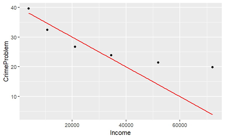
The mathematical function drawn is not a very good match to the data, but this reading is about how to draw graphs, not how to choose a family of functions or find parameters! If, when plotting your data, you prefer to set the limits of the axes to something of your own choice, you can do this. For instance:
gf_point(
  CrimeProblem ~ Income, data = Housing) %>%
  slice_plot(
    40 - Income / 2000 ~ Income, color = "blue") %>%
  gf_lims(
    x = range(0,100000),
    y=range(0,50))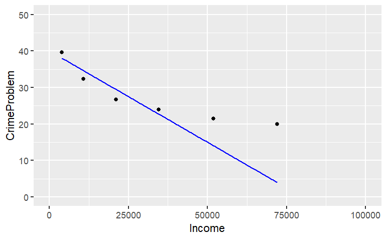
Properly made scientific graphics should have informative axis names. You can set the axis names directly using gf_labs:
gf_point(
  CrimeProblem ~ Income, data=Housing) %>%
  gf_labs(x= "Income Bracket ($US per household)/year",
          y = "Fraction of Households",
          main = "Crime Problem") %>%
  gf_lims(x = range(0,100000), y = range(0,50))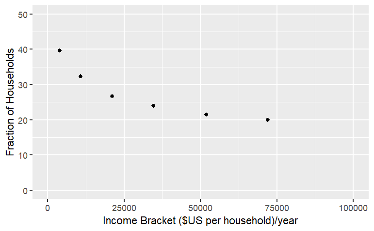
Notice the use of double-quotes to delimit the character strings, and how \(x\) and \(y\) are being used to refer to the horizontal and vertical axes respectively.
Make each of these plots:
Prof. Stan Wagon (see http://stanwagon.com) illustrates curve fitting using measurements of the temperature (in degrees C) of a cup of coffee versus time (in minutes):
s = read.csv(
  "http://www.mosaic-web.org/go/datasets/stan-data.csv")
gf_point(temp ~ time, data=s)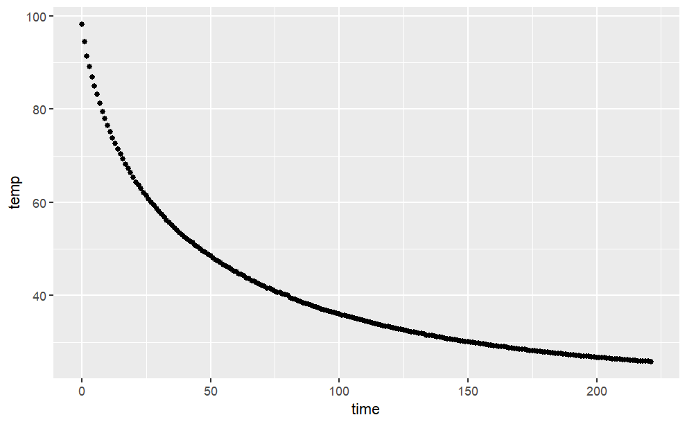
h = read.csv(
  "http://www.mosaic-web.org/go/datasets/hawaii.csv")
gf_point(water ~ time, data=h)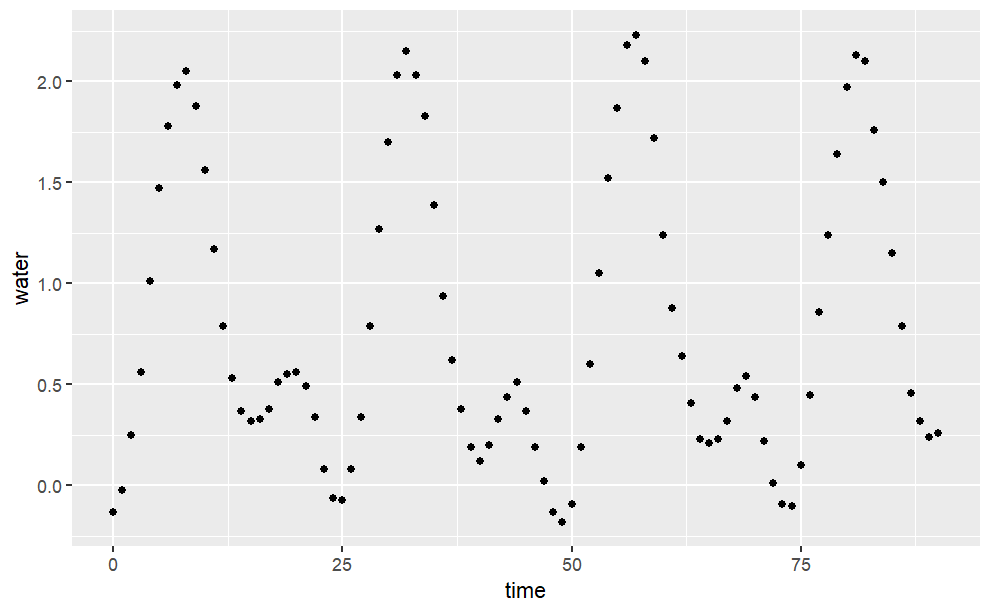
Describe in everyday English the pattern you see in the tide data:
Construct the R commands to duplicate each of these plots. Hand in your commands (not the plot):
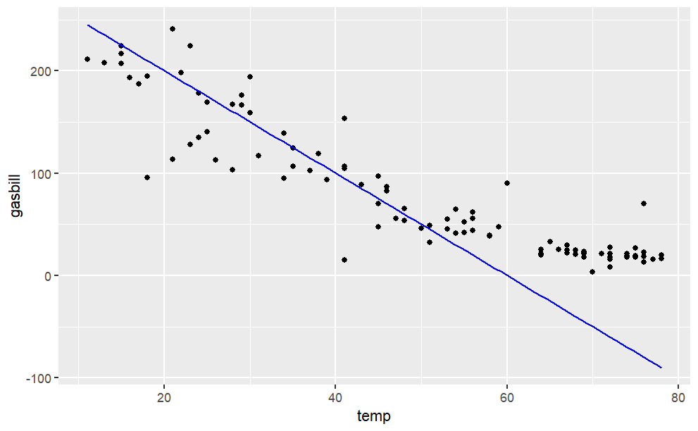
The data file "utilities.csv" has utility records for a house in St. Paul, Minnesota, USA. Make this plot, including the labels:
Here is your dataset: http://www.mosaic-web.org/go/datasets/utilities.csv
From the "utilities.csv" data file, make this plot of household monthly bill for natural gas versus average temperature. The line has slope \(−5\) USD/degree and intercept \(300\) USD.
You’ve already seen how to plot a graph of a function of one variable, for instance:
slice_plot(
  95 - 73*exp(-.2*t) ~ t,
  domain(t = 0:20) )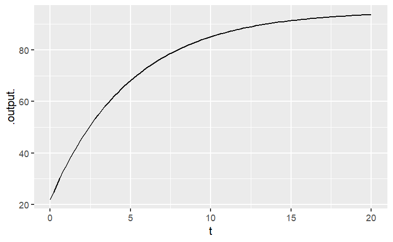
This lesson is about plotting functions of two variables. For the most part, the format used will be a contour plot. You use contour_plot() to plot with two input variables. You need to list the two variables on the right of the + sign, and you need to give a range for each of the variables. For example:
contour_plot(
  sin(2*pi*t/10)*exp(-.2*x) ~ t & x,
  domain(t = range(0,20), x = range(0,10)))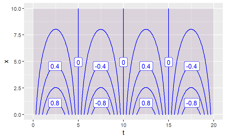
Each of the contours is labeled, and by default the plot is filled with color to help guide the eye. If you prefer just to see the contours, without the color fill, use the tile=FALSE argument.
contour_plot(
  sin(2*pi*t/10)*exp(-.2*x) ~ t & x,
  domain(t=0:20, x=0:10))
Occasionally, people want to see the function as a surface, plotted in 3 dimensions. You can get the computer to display a perspective 3-dimensional plot by using the interactive_plot() function. As you’ll see by mousing around the plot, it is interactive.
interactive_plot(
   sin(2*pi*t/10)*exp(-.5*x) ~ t & x,
   domain(t = 0:20, x = 0:10))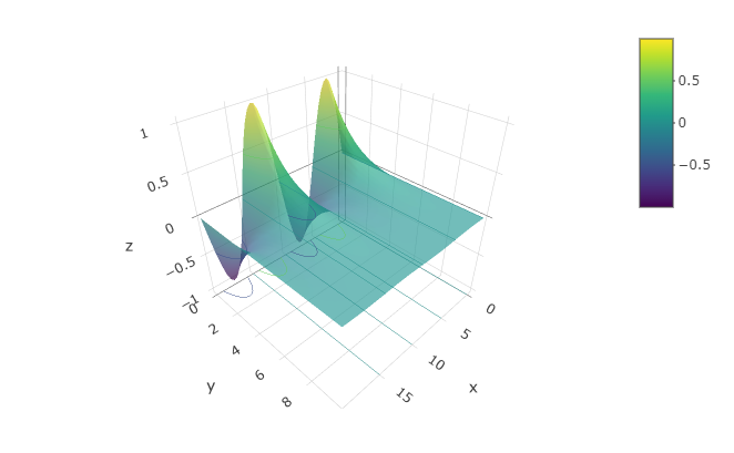
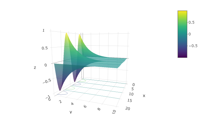
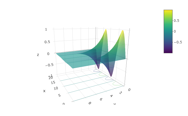
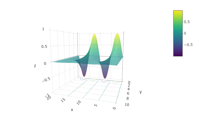
It’s very hard to read quantitative values from a surface plot — the contour plots are much more useful for that. On the other hand, people seem to have a strong intuition about shapes of surfaces. Being able to translate in your mind from contours to surfaces (and vice versa) is a valuable skill. To create a function that you can evaluate numerically, construct the function with makeFun(). For example:
g <- makeFun(
  sin(2*pi*t/10)*exp(-.2*x) ~ t & x)
contour_plot(
  g(t, x) ~ t + x,
  domain(t=0:20, x=0:10))
g(x = 4, t = 7)[1] -0.4273372Make sure to name the arguments explicitly when inputting values. That way you will be sure that you haven’t reversed them by accident. For instance, note that this statement gives a different value than the above:
g(4, 7)[1] 0.1449461The reason for the discrepancy is that when the arguments are given without names, it’s the position in the argument sequence that matters. So, in the above, 4 is being used for the value of t and 7 for the value of x. It’s very easy to be confused by this situation, so a good practice is to identify the arguments explicitly by name:
g(t = 7, x = 4)Describe the shape of the contours produced by each of these functions. (Hint: Make the plot! Caution: Use the mouse to make the plotting frame more-or-less square in shape.)
contour_plot(
  sqrt( (v-3)^2 + 2*(w-4)^2 ) ~ v & w,
  domain(v=0:6, w=0:6))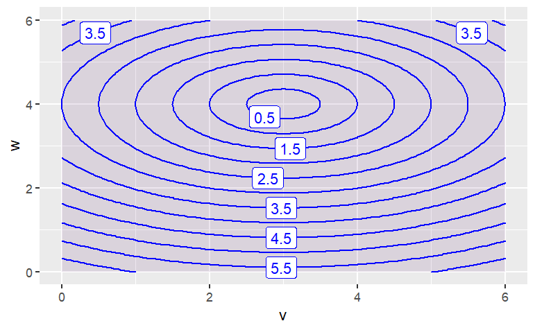
The function has contours that are {Parallel Lines,Concentric Circles,Concentric Ellipses,X Shaped}
contour_plot(
  sqrt( (v-3)^2 + (w-4)^2 ) ~ v & w,
  domain(v=0:6, w=0:6))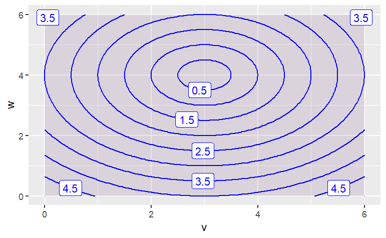
The function has contours that are {Parallel Lines,Concentric Circles, Concentric Ellipses, X Shaped}
contour_plot(
  6*v - 3*w + 4 ~ v & w,
  domain(v=0:6, w=0:6))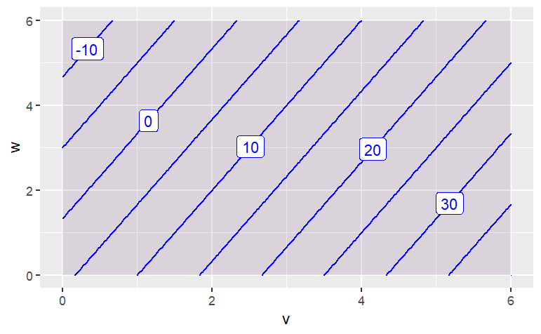
The function has contours that are:{Parallel Lines,Concentric Circles,Concentric Ellipses,X Shaped}}
Give the parameterizations of exponentials, sines, power laws. The idea is to make the arguments to the mathematical functions dimensionless. Parameters and logarithms – You can take the log of anything you like. The units show up as a constant
EXPLAIN hyper-parameter. It’s a number that governs the shape of the function, but it can be set arbitrarily and still match the data. Hyper-parameters are not set directly by the data.
Mathematical models attempt to capture patterns in the real world. This is useful because the models can be more easily studied and manipulated than the world itself. One of the most important uses of functions is to reproduce or capture or model the patterns that appear in data.
Sometimes, the choice of a particular form of function — exponential or power-law, say — is motivated by an understanding of the processes involved in the pattern that the function is being used to model. But other times, all that’s called for is a function that follows the data and that has other desirable properties, for example is smooth or increases steadily.
“Smoothers” and “splines” are two kinds of general-purpose functions that can capture patterns in data, but for which there is no simple algebraic form. Creating such functions is remarkably easy, so long as you can free yourself from the idea that functions must always have formulas.
Smoothers and splines are defined not by algebraic forms and parameters, but by data and algorithms. To illustrate, consider some simple data. The data set Loblolly contains 84 measurements of the age and height of loblolly pines.
gf_point(height ~ age, data=datasets::Loblolly)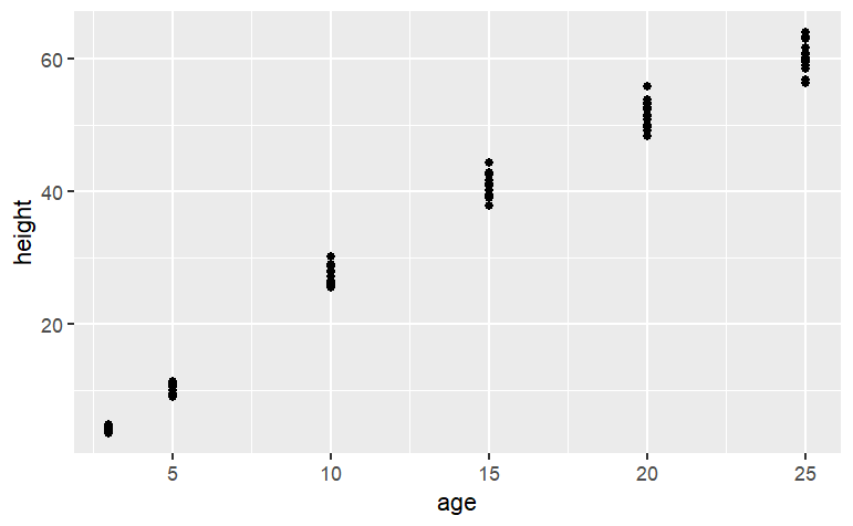
Several three-year old pines of very similar height were measured and tracked over time: age five, age ten, and so on. The trees differ from one another, but they are all pretty similar and show a simple pattern: linear growth at first which seems to low down over time. It might be interesting to speculate about what sort of algebraic function the loblolly pines growth follows, but any such function is just a model. For many purposes, measuring how the growth rate changes as the trees age, all that’s needed is a smooth function that looks like the data. Let’s consider two:
f1 <- spliner(height ~ age, data = datasets::Loblolly)f2 <- connector(height ~ age, data = datasets::Loblolly)The definitions of these functions may seem strange at first — they are entirely defined by the data: no parameters! Nonetheless, they are genuine functions and can be worked with like other functions. For example, you can put in an input and get an output:
f1(age = 8)[1] 20.68193f2(age = 8)[1] 20.54729You can graph them:
f1 <- spliner(height ~ age, data = datasets::Loblolly)
f2 <- connector(height ~ age, data = datasets::Loblolly)
gf_point(height ~ age, data = datasets::Loblolly) %>%
  slice_plot(f1(age) ~ age) %>%
  slice_plot(f2(age) ~ age, color="red",
             findZeros(f1(age) - 35 ~ age,
xlim=range(0,30))) 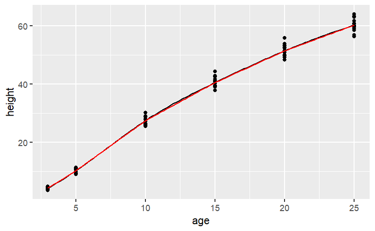
You can even “solve” them, for instance finding the age at which the height will be 35 feet:
In all respects, these are perfectly ordinary functions. All respects but one: there is no simple formula for them. You’ll notice this if you ever try to look at the computer-language definition of the functions:
f2## function (age)
## {
## x <- get(fnames[2])
## if (connect)
## SF(x)
## else SF(x, deriv = deriv)
## }
## <environment: 0x7ff1bf85ec18>There’s almost nothing here to tell the reader what the body of the function is doing. The definition refers to the data itself which has been stored in an “environment.” These are computer-age functions, not functions from the age of algebra. As you can see, the spline and linear connector functions are quite similar, except for the range of inputs outside of the range of the data. Within the range of the data, however, both types of functions go exactly through the center of each age-group. Splines and connectors are not always what you will want, especially when the data are not divided into discrete groups, as with the loblolly pine data. For instance, the trees.csv data set is measurements of the volume, girth, and height of black cherry trees. The trees were felled for their wood, and the interest in making the measurements was to help estimate how much usable volume of wood can be gotten from a tree, based on the girth (that is, circumference) and height. This would be useful, for instance, in estimating how much money a tree is worth. However, unlike the loblolly pine data, the black cherry data does not involve trees falling nicely into defined groups.
Cherry <- datasets::trees
gf_point(Volume ~ Girth, data = Cherry)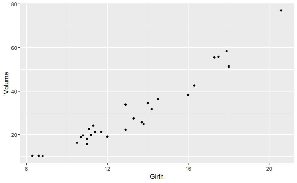
It’s easy enough to make a spline or a linear connector:
g1 = spliner(Volume ~ Girth, data = Cherry)
g2 = connector(Volume ~ Girth, data = Cherry)
slice_plot(g1(x) ~ x, domain(x = 8:18)) %>%
  slice_plot(g2(x) ~ x, color ="red") %>%
  gf_point(Volume ~ Girth, data = Cherry) %>%
  gf_labs(x = "Girth (inches)")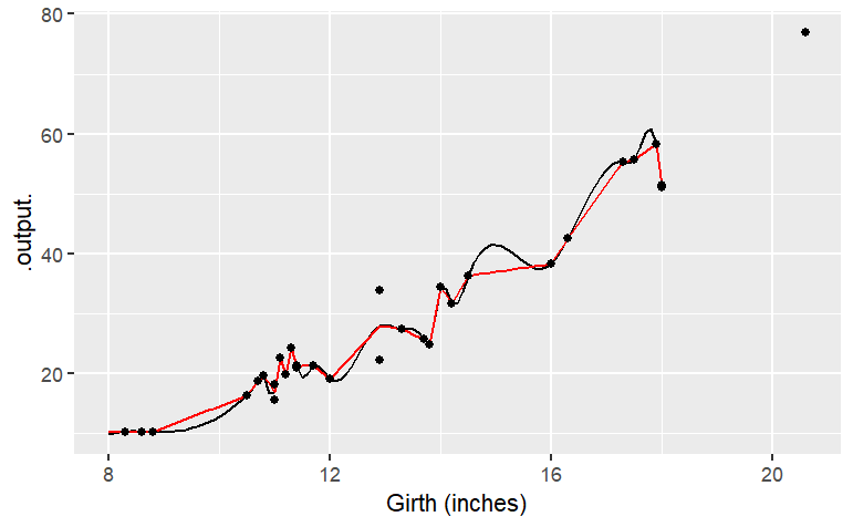
The two functions both follow the data … but a bit too faithfully! Each of the functions insists on going through every data point. (The one exception is the two points with girth of 13 inches. There’s no function that can go through both of the points with girth 13, so the functions split the difference and go through the average of the two points.) The up-and-down wiggling is of the functions is hard to believe. For such situations, where you have reason to believe that a smooth function is more appropriate than one with lots of ups-and-downs, a different type of function is appropriate: a smoother.
g3 <- smoother(Volume ~ Girth, data = Cherry, span=1.5)
gf_point(Volume~Girth, data=Cherry) %>%
  slice_plot(g3(Girth) ~ Girth) %>%
  gf_labs(x = "Girth (inches)")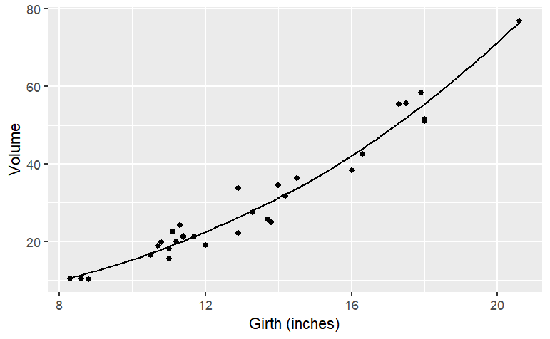
smoothers() are well named: they construct a smooth function that goes close to the data. You have some control over how smooth the function should be. The hyper-parameter span governs this:
g4 <- smoother(Volume ~ Girth, data=Cherry, span=1.0)
gf_point(Volume~Girth, data = Cherry) %>%
  slice_plot(g4(Girth) ~ Girth) %>%
  gf_labs(x = "Girth (inches)", y = "Wood volume")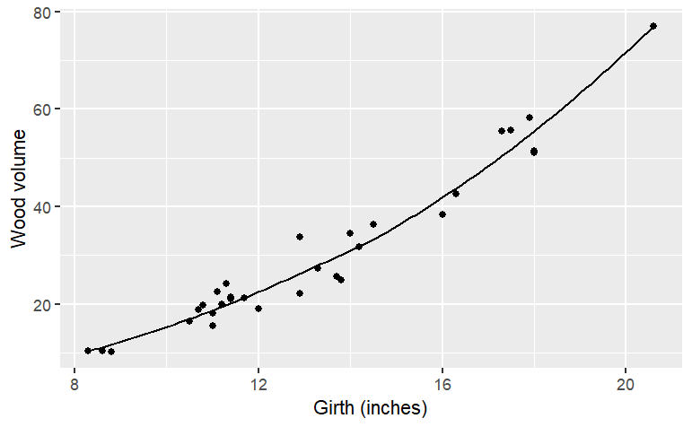
Of course, often you will want to capture relationships where there is more than one variable as the input. Smoothers do this very nicely; just specify which variables are to be the inputs.
g5 <- smoother(Volume ~ Girth+Height,
               data = Cherry, span = 1.0)
gf_point(Height ~ Girth, data = Cherry) %>%
  contour_plot(g5(Girth, Height) ~ Girth + Height) %>%
  gf_labs(x = "Girth (inches)",
          y = "Height (ft)",
          title = "Volume (ft^3)")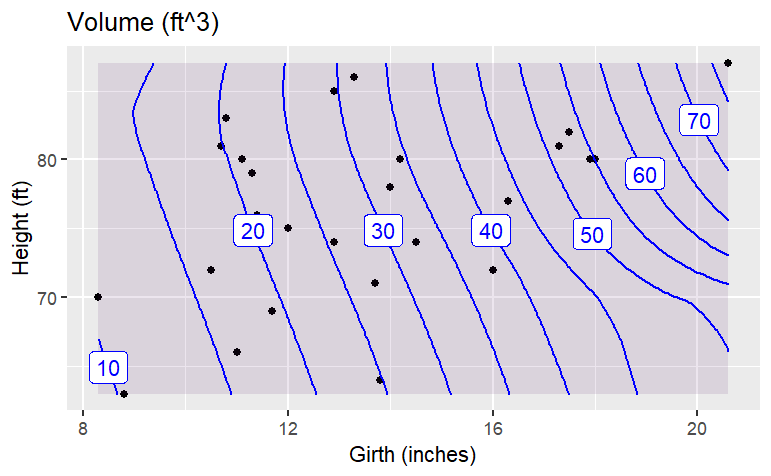
When you make a smoother or a spline or a linear connector, remember these rules:
You need a data frame that contains the data.
You use the formula with the variable you want as the output of the function on the left side of the tilde, and the input variables on the right side.
The function that is created will have input names that match the variables you specified as inputs. (For the present, only smoother will accept more than one input variable.)
The smoothness of a smoother function can be set by thespan argument. A span of 1.0 is typically pretty smooth.The default is 0.5.
When creating a spline, you have the option of declaring monotonic=TRUE. This will arrange things to avoid extraneous bumps in data that shows a steady upward pattern or a steady downward pattern.
When you want to plot out a function, you need of course to choose a range for the input values. It’s often sensible to select a range that corresponds to the data on which the function is based. You can find this with the range() command, e.g.
range(Cherry$Height)Much of the content of high-school algebra involves “solving.” In the typical situation, you have an equation, say
\[ y= 3x+2 \]
and you are asked to “solve” the equation for \(x\). This involves rearranging the symbols of the equation in the familiar ways, e.g., moving the \(2\) to the right hand side and dividing by the \(3\). High school students are also taught a variety of ad hoc techniques for solving in particular situations. For example, the quadratic equation \(ax^2+bx+c=0\) can be solved by application of the procedures of “factoring,” or “completing the square,” or use of the quadratic formula
\[ x= \dfrac{-b \pm\sqrt{b^2-4ac}}{2a} \]
Parts of this formula can be traced back to at least the year 628 in the writings of Brahmagupta, an Indian mathematician, but the complete formula seems to date from Simon Stevin in Europe in 1594, and was published by René Descartes in 1637.
For some problems, students are taught named operations that involve the inverse of functions. For instance, to solve \(\sin(x)=y\), one simply writes down \(x= \arcsin y\) without any detail on how to find \(\arcsin\) beyond “use a calculator” or, in the old days, “use a table from a book.”
With all of this emphasis on procedures such as factoring and moving symbols back and forth around an = sign, students naturally ask, “How do I solve equations in R?”
The answer is surprisingly simple, but to understand it, you need to have a different perspective on what it means to “solve” and where the concept of “equation” comes in.
The general form of the problem that is typically used in numerical calculations on the computer is that the equation to be solved is really a function to be inverted. That is, for numerical computation, the problem should be stated like this:
You have a function \(f(x)\). You happen to know the form of the function \(f\) and the value of the output \(y\)for some unknown input value \(x\). Your problem is to find the input \(x\) given the function \(f\) and the output value \(y\).
One way to solve such problems is to find the inverse of \(f\) This is often written \(f^{-1}\) (which many students understandably but mistakenly take to mean \(\frac{1}{f(x)}\). But finding the inverse of \(f\) can be very difficult and is overkill. Instead, the problem can be handled by finding the zeros of \(f\).
If you can plot out the function \(f(x)\) for a range of \(x\), you can easily find the zeros. Just find where the \(x\) where the function crosses the \(y\)-axis. This works for any function, even ones that are so complicated that there aren’t algebraic procedures for finding a solution.
To illustrate, consider the function \(g( )\)
g <- makeFun(sin(x^2)*cos(sqrt(x^4 + 3 )-x^2) - x + 1 ~ x)
slice_plot(g(x) ~ x, domain(x = -3:3)) %>%
  gf_hline(yintercept  = 0, color = "red")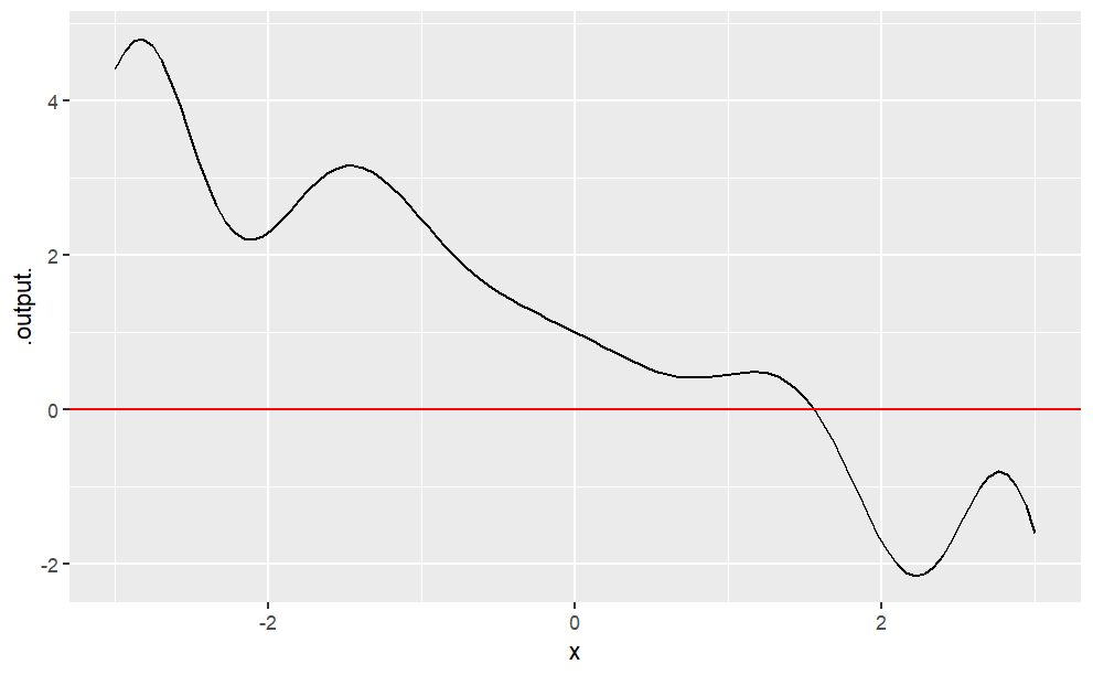
You can see easily enough that the function crosses the \(y\) axis somewhere between \(x=1\) and \(x=2\). You can get more detail by zooming in around the approximate solution:
slice_plot(g(x) ~ x, domain(x=1:2)) %>%
  gf_hline(yintercept = 0, color = "red")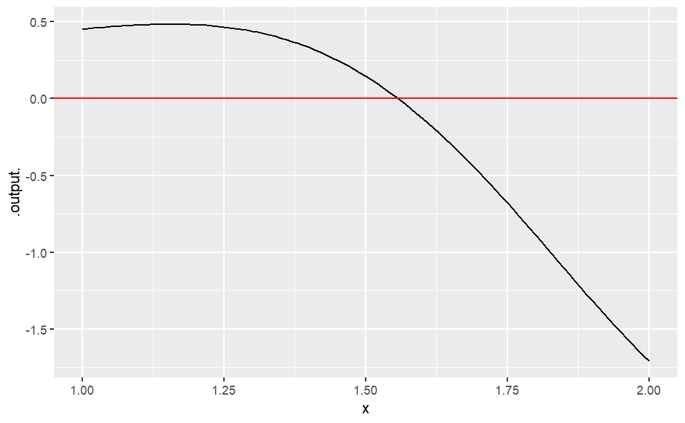
The crossing is at roughly \(x \approx1.6\) You could, of course, zoom in further to get a better approximation. Or, you can let the software do this for you:
findZeros(g(x) ~ x, xlim = range(1, 2))The argument xlim is used to state where to look for a solution. (Due to a software bug, it’s always called xlim even if you use a variable other than x in your expression.) You need only have a rough idea of where the solution is. For example:
findZeros(g(x) ~ x, xlim = range(-1000, 1000))findZeros() will only look inside the interval you give it. It will do a more precise job if you can state the interval in a narrow way.