Code
N <- 10000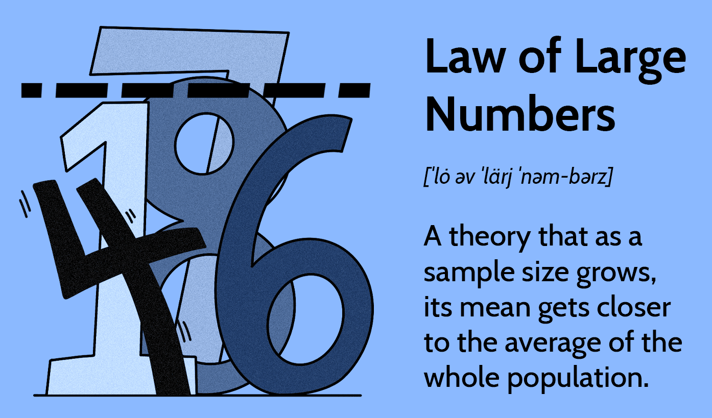
set.seed(1963) # added for the example - comment out for testDefinition: The Law of Large Numbers states that as the sample size increases (or as the number of trials in an experiment increases), the sample mean (or what) converges in probability to the population mean. In simpler terms, as you take more observations from a population, the average of those observations tends to get closer to the true average of the entire population.
Key Point: LLN is concerned with the behavior of sample averages as the sample size grows, and it emphasizes the stability and reliability of sample statistics as estimates of population parameters.
In probability theory, the law of large numbers (LLN) is a theorem that describes the result of performing the same experiment a large number of times. According to the law, the average of the results obtained from a large number of trials should be close to the expected value, and will tend to become closer as more trials are performed.
The Law of Large Numbers (LLN) is a fundamental theorem in probability theory and statistics. It describes the behavior of the sample mean of a random variable as the sample size increases.
N.B: It doesn’t describe the distribution of individual samples; rather, it focuses on the convergence properties of the sample mean to the population mean.
Weak Law of Large Numbers (WLLN): The Weak Law of Large Numbers states that as the sample size (the number of observations or trials) increases, the sample mean (average) of those observations will converge in probability to the expected value (mean) of the random variable. In other words, as you collect more data, the sample mean becomes a better and better estimate of the true population mean.
Mathematically, if X1, X2, …, Xn are independent and identically distributed random variables with a common mean (μ) and finite variance, then as n (the sample size) approaches infinity:
\(\displaystyle\frac{(X_1+X_2+…+X_n)}{n}\) converges in probability to \(\mu\) .
Strong Law of Large Numbers (SLLN): The Strong Law of Large Numbers is a more powerful version of the LLN. It states that as the sample size increases, the sample mean converges almost surely (with probability 1) to the expected value of the random variable. This means that not only does the sample mean converge in probability to the population mean, but it almost surely equals the population mean for sufficiently large sample sizes.
Mathematically, for the same conditions as in the WLLN, the SLLN states that:
\(\displaystyle\frac{(X_1+X_2+…+X_n)}{n}\) converges almost surely to \(\mu\) as \(n \to \infty\).
The LLN is a fundamental concept in statistics and provides a theoretical basis for many statistical techniques. It underlines the idea that as you collect more and more data, your sample statistics (such as the sample mean) become increasingly reliable estimators of the population parameters (such as the population mean).
A fair coin flip should be heads 50% of the times.
N represents the total number of observations, or in this example, coin flips.Comment out set.seed() to achieve randomness on subsequent runs.
N <- 10000
set.seed(1963) # added for the example - comment out for testNow we will set 3 variables to simulate the coin flips.
flip_outcome - stores the sample flips as a 0 or 1. The number of flips will me set by the value of N set previously.
flip_cumulative_sum - stores a running total of the occurrences of a value of “1”, say heads.
running_avg - stores the running avg with each flip.
Recall
sample() : sample takes a sample of the specified size from the elements of x using either with or without replacement.
cumsum() :Returns a vector whose elements are the cumulative sums, products, minima or maxima of the elements of the argument.
flip_outcome <- sample(x = 0:1,
# either a vector of one or more elements from which to
#choose, or a positive integer.
                    size = N,
# a non-negative integer giving the number of items to choose.
                 replace = T
#  should sampling be with replacement?
                      )
Explore what you just created.
flip_outcome[1:10]flip_cumulative_sum <- cumsum(flip_outcome)
flip_cumulative_sum[1:10]running_avg <- flip_cumulative_sum/(1:N)
running_avg[1:10]Assign the running statistics gathered to the r.stats variable.
Show the results (should limit to approx 100 observations in this list)
r.stats <- round(x = cbind(flip_outcome,
                           flip_cumulative_sum,
                           running_avg
                           ),
                 digits =  3)[1:10,]

# 10 represents the number of observations to display
#to look at the results as they are run.
#It should not exceed 100 for practical purposes.

print(r.stats)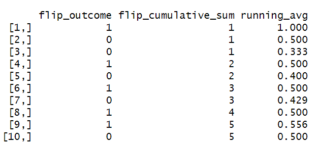
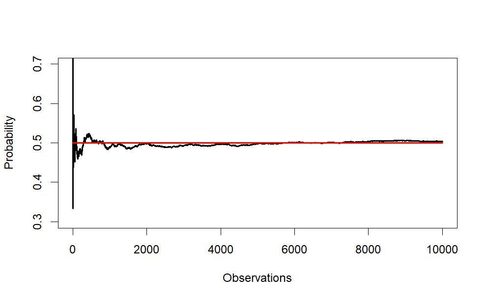
Create a plot chart to illustrate how the means of the sample approximately equals the population with large sample sizes. scipen used to influence the x axis to use whole numbers for large observation counts
The plot uses line charts to reflect
the running averages of the coin flips and
the expected average of the population (.5).
options() Allow the user to set and examine a variety of global options which affect the way in which R computes and displays its results.
lines() A generic function taking coordinates given in various ways and joining the corresponding points with line segments.
options(scipen = 10)
# integer. A penalty to be applied when deciding to
#print numeric values in fixed or exponential notation.
#Positive values bias towards fixed and negative
#towards scientific notation: fixed notation will be preferred unless
#it is more than scipen digits wider.

plot(x    = running_avg ,
     ylim = c(.30, .70),
     type = "l",
     xlab = "Observations",
     ylab = "Probability",
     lwd  = 2
     )

# to add the 50% chance line
lines(x = c(0,N),
      y = c(.50,.50),
      col="red",
      lwd = 2
      )
lines() : A generic function taking coordinates given in various ways and joining the corresponding points with line segments.
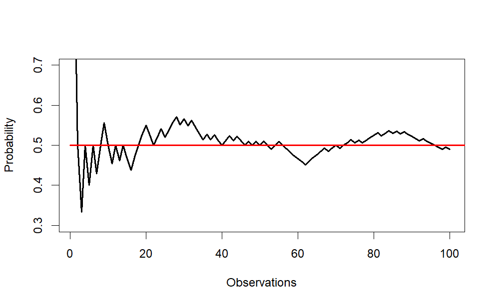
plot(x    = running_avg[1:100],
     ylim = c(.30, .70),
     type = "l",
     xlab = "Observations",
     ylab = "Probability",
     lwd  = 2
     )

# to add the 50% chance line
lines(x = c(0,N),
      y = c(.50,.50),
      col="red",
      lwd = 2
      )
library(knitr)
knitr::opts_chunk$set(tidy=T,
               fig.width=10,
               fig.height=5,
               fig.align='left',
               warning=FALSE,
               message=FALSE,
               echo=TRUE)
options(width = 120)
library(ggplot2)
library(scales)Create a function to generate data simulating tosses of a coin.
tossCoin = function(n=30, p=0.5) {

# create a probability distribution,
#a vector of outcomes (H/T are coded using 0/1)
# and their associated probabilities
  outcomes = c(0,1) # sample space
  probabilities = c(1-p,p)

# create a random sample of n flips; this could also be done with
# the rbinom() function, but sample() is perhaps more useful
  flips = sample(outcomes,n,replace=T,prob=probabilities)

  # now create a cumulative mean vector
  cum_sum = cumsum(flips)
  index = c(1:n)
  cum_mean = cum_sum / index

  # now combine the index, flips and cum_mean vectors
  # into a data frame and return it
  # return(data.frame(index,flips,cum_mean))
  return(data.frame(index,cum_mean))
}
Plot the data to demonstrate how the cumulative sample mean converges on the expected value when the sample gets large.
ggplotCoinTosses = function(n=30, p=.50) {
  # visualize how cumulative average converges on p
  # roll the dice n times and calculate means
  trial1 = tossCoin(n,p)
  max_y = ceiling(max(trial1$cum_mean))
  if (max_y < .75) max_y = .75
  min_y = floor(min(trial1$cum_mean))
  if (min_y > .4) min_y = .4

  # calculate last mean and standard error
  last_mean = round(trial1$cum_mean[n],9)

  # plot the results together
  plot1 = ggplot(trial1, aes(x=index,y=cum_mean)) +
    geom_line(colour = "blue") +
    geom_abline(intercept=0.5,slope=0, color = 'red', size=.5) +
    theme(plot.title = element_text(size=rel(1.5)),
          panel.background = element_rect()) +
    labs(x = "n (number of tosses)",
         y = "Cumulative Average") +
    scale_y_continuous(limits = c(min_y, max_y)) +
    scale_x_continuous(trans = "log10",
                       breaks = trans_breaks("log10",function(x) 10^x),
                       labels = trans_format("log10",math_format(10^.x))) +
    annotate("text",
             label=paste("Cumulative mean =", last_mean,
                         "\nEV =",  p,
                         "\nSample size =", n),
             y=(max_y - .20),
             x=10^(log10(n)/2), colour="darkgreen") +
    annotate("text",
           label=paste("P(Heads) with Fair Coin = 0.50"),
           y=(max_y - .80),
           x=10^(log10(n)/2), colour="red")

  return(plot1)
}
# call the function; let's use a fair coin
ggplotCoinTosses(100000, .50)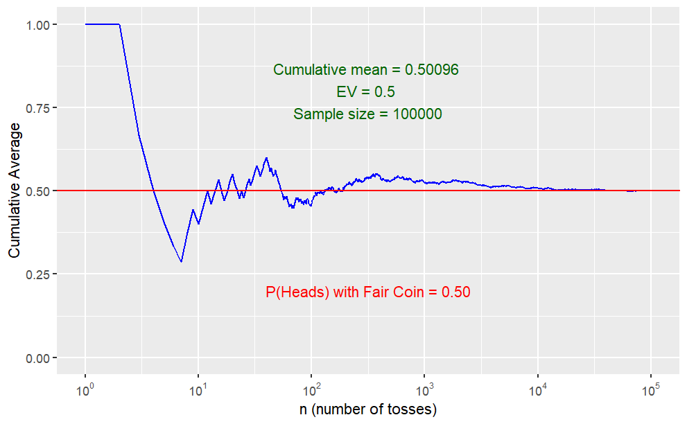
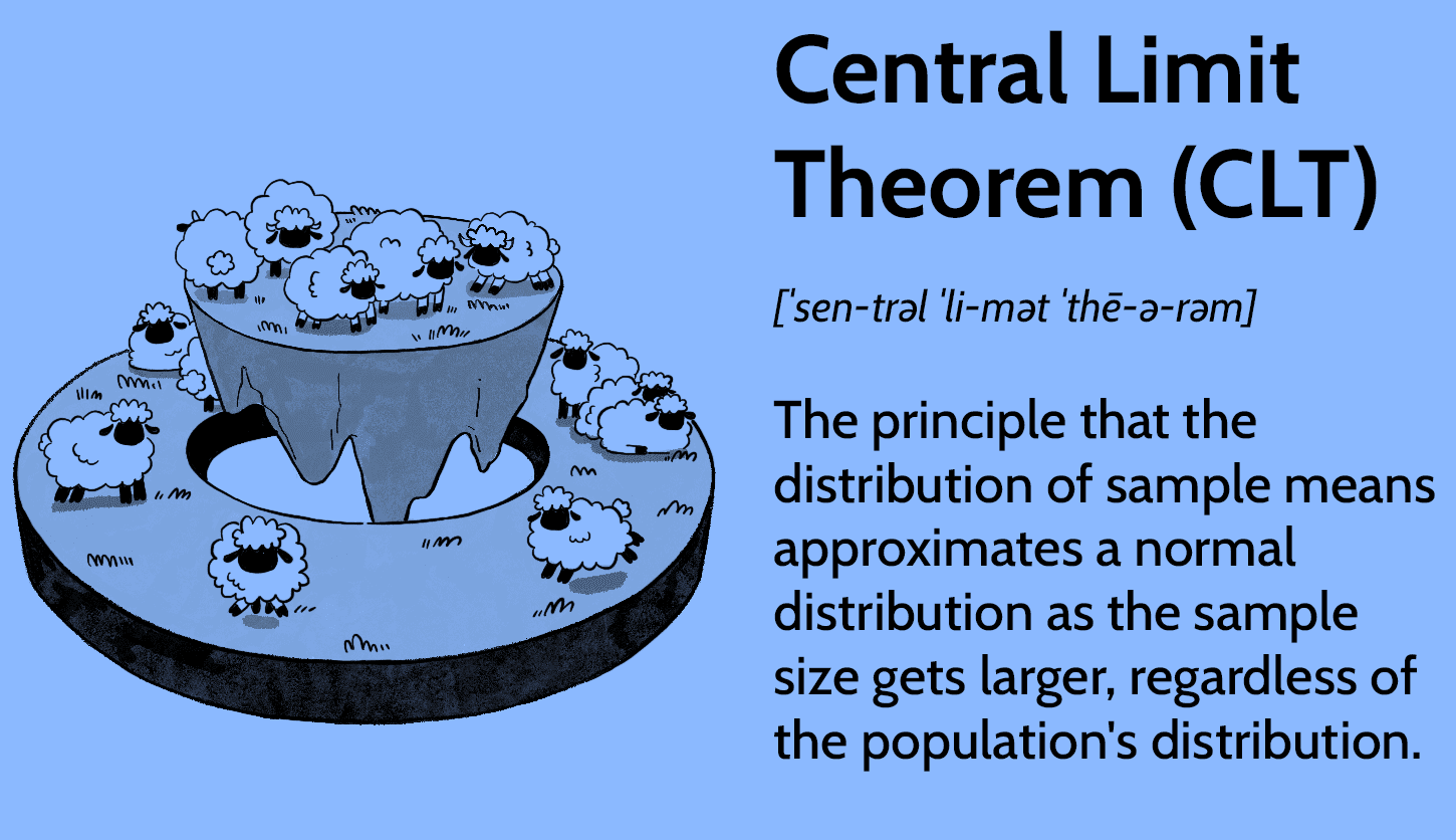
Definition: The Central Limit Theorem states that, regardless of the distribution of the population, the sampling distribution of the sample mean (or any sufficiently large sample statistic) will be approximately normally distributed. This holds true as long as the sample size is large enough.
Key Point: CLT is concerned with the shape of the distribution of the sample mean, suggesting that it becomes normal as the sample size increases, irrespective of the original distribution of the population.
The Central Limit Theorem basically says that all sampling distributions turn out to be bell-shaped.
If you have a sufficiently large sample size drawn from a population with any shape of distribution (not necessarily normal), the distribution of the sample mean will be approximately normally distributed.
Specifically, the Central Limit Theorem states the following:
Let \(X_1, X_2, \ldots, X_n\) be a sequence of independent and identically distributed (i.i.d.) random variables with a mean \(\mu\) and a finite standard deviation \(\sigma\). If \(n\) is sufficiently large, then the distribution of the sample mean \(\bar{X}\) (the average of the sample) will be approximately normally distributed with a mean \(\mu\) and a standard deviation \(\displaystyle \frac{\sigma}{\sqrt{n}}.\) Mathematically, this can be expressed as:
\[ \bar{X} \sim \Bigg(\mu,\frac{\sigma}{\sqrt{n}} \Bigg) \]
This is a powerful result because it allows statisticians to make inferences about population parameters using the normal distribution, even when the underlying population distribution is not normal. The larger the sample size (n), the closer the distribution of the sample mean will be to a normal distribution, regardless of the original distribution of the population.
Both LLN and CLT are concerned with the behavior of sample statistics, particularly the sample mean, as sample size increases.
Both are fundamental concepts in statistics and play crucial roles in inferential statistics.
Focus:
LLN: Focuses on the behavior of the sample mean as the sample size increases and how it converges to the population mean.
CLT: Focuses on the distribution of the sample mean, stating that it becomes approximately normal with a large sample size, regardless of the population distribution.
Assumption:
LLN: Assumes the existence of the population mean and investigates the behavior of the sample mean as the sample size increases.
CLT: Does not necessarily assume the existence of a population mean; it deals with the distribution of the sample mean.
In summary, LLN deals with the convergence of sample statistics to population parameters, while CLT deals with the distributional properties of sample statistics, particularly the sample mean.
In other words, the CLT includes the LLN as a special case.
The Law of Large Numbers (LLN) is a fundamental concept that describes the behavior of sample averages as the sample size increases, stating that the sample mean converges in probability to the population mean. The focus of LLN is on the convergence of sample statistics to population parameters.
The Central Limit Theorem (CLT) is a more powerful and general result. It states that, under certain conditions, the distribution of the sum (or average) of a large number of independent, identically distributed random variables approaches a normal distribution, regardless of the shape of the original population distribution. This implies that the sample mean, for a sufficiently large sample size, will be approximately normally distributed.
Here’s the relationship:
In essence, the LLN can be viewed as a special case of the more general CLT when applied to the sample mean. Therefore, while LLN provides insights into the convergence of sample means, CLT extends these insights to describe the distributional properties of sample means as the sample size becomes large.
The Mosaic package was created by statistics instructors to help students learn the coding in R. Commands are streamlined to be more intuitive. Execute the code block below to load Mosaic (required each session).
library(mosaic)A sampling distribution is created by repeatedly drawing samples of the same size from an underlying distribution. In the examples below, n is the sample size for each individual draw, and Trials is the number of samples drawn.
Key Idea: the mean of a sampling distribution will be bell-shaped, regardless of the underlying distribution. The next dozen examples show the bell-shape sampling distribution emerging in the histograms as the number of trials increases.
coins = do(50) * rflip(30)
histogram(~heads, data = coins,
          width = 1,
          fit = "normal")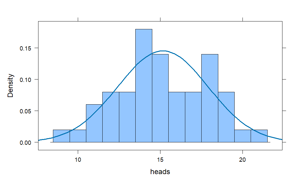
The bell-shape is apparent but falls short of perfection. With larger sample sizes, the bars in the histogram will match up better with the envelope of the superimposed bell curve.
coins = do(200) * rflip(20)
histogram(~heads, data = coins,
          width = 1,
          fit = "normal")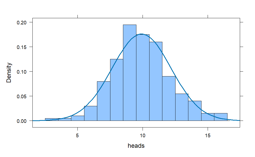
coins = do(1000) * rflip(20)
histogram(~heads, data = coins,
          width = 1,
          fit = "normal")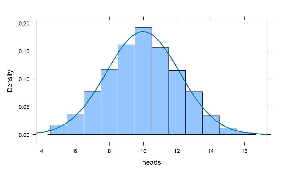
With a thousand trials, we observe a near-perfect bell-shape emerging in the histogram.
coins = do(50) * rflip(20, prob = .8)
histogram(~heads, data = coins,
          width = 1,
          fit = "normal")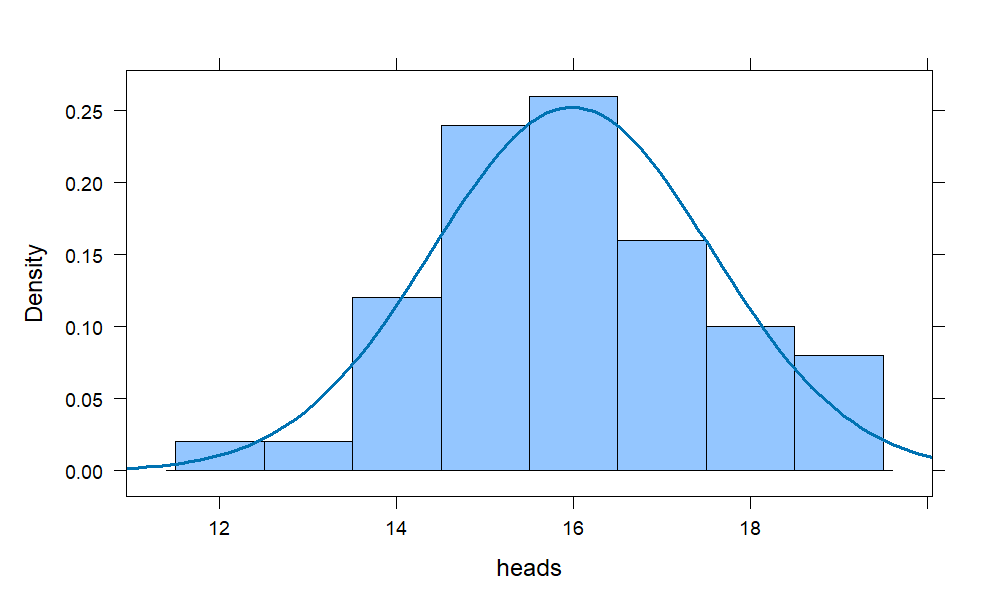
coins = do(200) * rflip(20, prob = .8)
histogram(~heads, data = coins,
          width = 1,
          fit = "normal")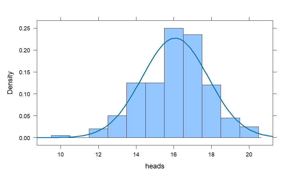
coins = do(1000) * rflip(20, prob = .8)
histogram(~heads, data = coins,
          width = 1,
          fit = "normal")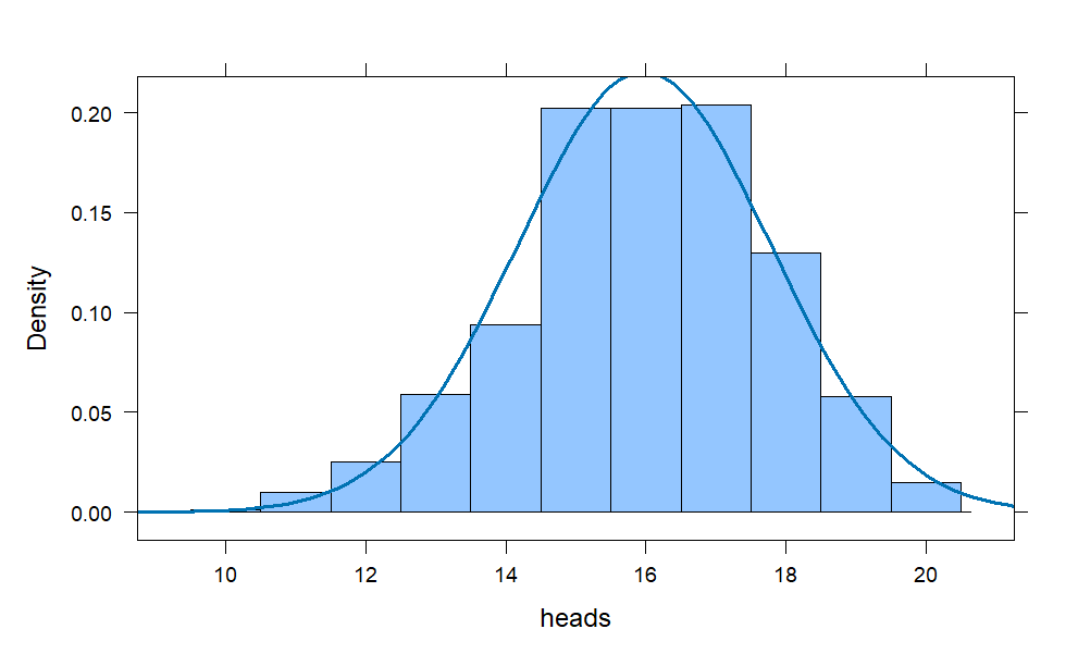
Notice the left tail of the histogram is slightly longer, but the bell-shape is nearly perfect and centered at 16 which is 80% of 20, as one would anticipate.
What about the following distribution: we roll a 6-sided die and take the square of the value showing. Then our underlying distribution will look very non-normal and skewed hard left.
barplot(c(1,4,9,16,25,36),space = 0, col = "red")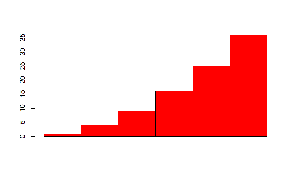
This isn’t a proper pdf because the y-axis is labeled in outcome values, not density, but the point was to show the shape, which it does.
d = do(50) * resample(1:6,20)
D = d^2
sumD = rowSums(D)
histogram(sumD ,
          width = 20,
          center = 300,
          fit = "normal")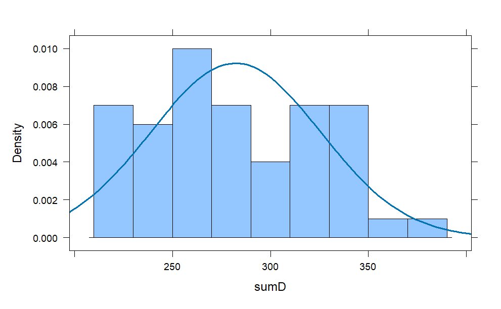
d = do(1000) * sample(1:6,20, replace = TRUE)
D = d^2
sumD = rowSums(D)
histogram(sumD ,
          width = 20,
          center = 300,
          fit = "normal")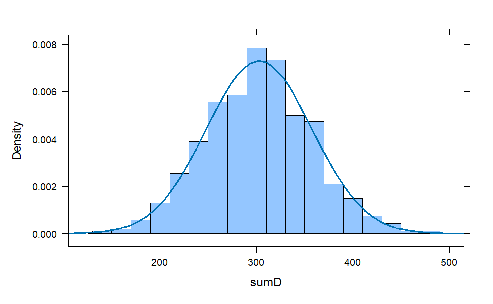
d = do(10000) * sample(1:6,20, replace = TRUE)
D = d^2
sumD = rowSums(D)
histogram(sumD ,
          width = 20,
          center = 300,
          fit = "normal")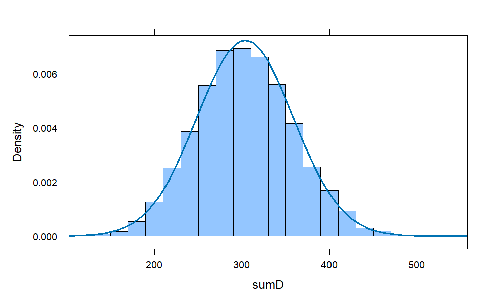
The sample theory is the study of relationships existing between a population and samples drawn from population.Consider all possible samples of size n that can be drawn from the population. For each sample, we can compute statistic like mean or a standard deviation, etc that will vary from sample to sample. This way we obtain a distribution called as the sampling distribution of a statistic. If the statisic is sample mean , then the distribution is called the sampling distribution of mean.
We can have sampling distribution of standard deviation, variance, medians, proportion etc.
The Central limit theorem states that the sampling distribution of the mean of any independent, random variable will be normal or near normal,regardless of underlying distribution.If the sample size is large enough,we get a nice bell shaped curve.
In other words, suppose you picked a sample from large number of independent and random observations and compute the arithmetic average of sample and do this exercise for n number of times. Then according to the central limit theorem the computed values of the average will be distributed according to the normal distribution (commonly known as a “bell curve”). We will try simulate this my theorem in examples below
Example 1: A fair die can be modelled with a discrete random variable with outcome 1 through 6, each with the equal probability of 1/6.
The expected value is \(\frac{1+2+3+4+5+6}{6} =3.5\)
Suppose you throw the die 10000 times and plot the frequency of each outcome. Here’s the r syntax to simulate the throwing a die 10000 times.
DieOutcome <- sample(1:6,10000, replace= TRUE)
hist(DieOutcome, col ="light blue")
abline(v=3.5, col = "red",lty=1)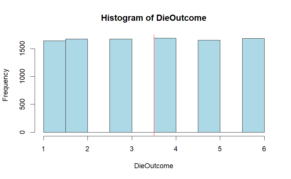
We will take samples of size 10 , from the above 10000 observation of outcome of die roll, take the arithmetic mean and try to plot the mean of sample. we will do this procedure k times (in this case k= 10000 )
x10 <- c()
k =10000
 for ( i in 1:k) {
 x10[i] = mean(sample(1:6,10, replace = TRUE))}
 hist(x10, col ="pink", main="Sample size =10",xlab ="Outcome of die roll")
 abline(v = mean(x10), col = "Red")
 abline(v = 3.5, col = "blue")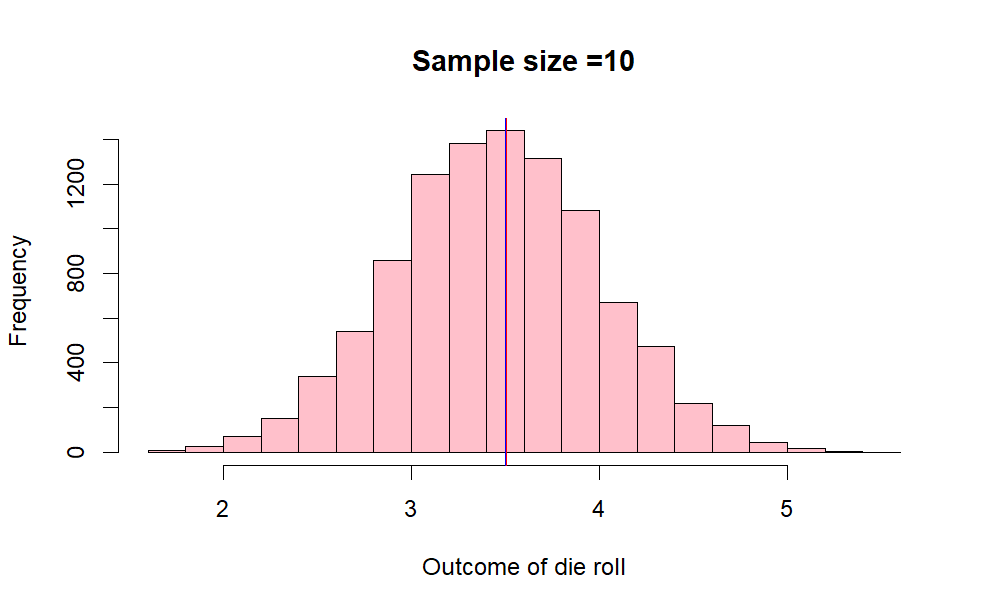
Sample Size
By theory , we know as the sample increases, we get better bell shaped curve. As the n apporaches infinity , we get a normal distribution. Lets do this by increasing the sample size to 30, 100 and 1000 in above example 1.
x30 <- c()
 x100 <- c()
 x1000 <- c()
 k =10000
 for ( i in 1:k){
 x30[i] = mean(sample(1:6,30, replace = TRUE))
 x100[i] = mean(sample(1:6,100, replace = TRUE))
 x1000[i] = mean(sample(1:6,1000, replace = TRUE))
 }
 par(mfrow=c(1,3))
 hist(x30, col ="green",main="n=30",xlab ="die roll")
 abline(v = mean(x30), col = "blue")

 hist(x100, col ="light blue", main="n=100",xlab ="die roll")
 abline(v = mean(x100), col = "red")

 hist(x1000, col ="orange",main="n=1000",xlab ="die roll")
 abline(v = mean(x1000), col = "red")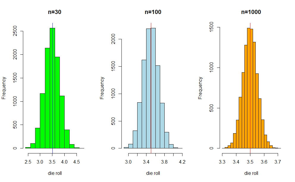
We will take another example
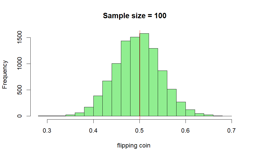
Example 2: A fair Coin
Flipping a fair coin many times the probability of getting a given number of heads in a series of flips should follow a normal curve, with mean equal to half the total number of flips in each series. Here 1 represent heads and 0 tails.
x <- c()
k =10000
 for ( i in 1:k) {
 x[i] = mean(sample(0:1,100, replace = TRUE))}
 hist(x, col ="light green", main="Sample size = 100",xlab ="flipping coin ")
 abline(v = mean(x), col = "red")