The Mystique of Snowflakes
Nature’s Fractal Masterpieces
Mathematics
R Programming
Nature’s Delicate Masterpieces
When winter blankets the world in a shimmering white coat, one of the most enchanting sights it brings is the snowflake. These delicate ice crystals fall from the sky in an endless array of intricate patterns, each one a tiny masterpiece of nature’s artistry.
But what exactly is a snowflake, and how does it form?
Snowflake Formation
At its most basic level, a snowflake is a tiny crystal of ice that forms when water vapor in the atmosphere condenses directly into ice without first becoming liquid. This process occurs in clouds where temperatures are well below freezing. As water vapor molecules come into contact with ice nuclei, which can be dust particles or even tiny salt crystals, they begin to arrange themselves into the hexagonal structure that characterizes ice crystals.
The shape of a snowflake is influenced by a variety of factors, including temperature, humidity, and wind patterns. As the crystal falls through the atmosphere, it may encounter different conditions at different altitudes, leading to the development of branches, plates, and other intricate structures.
Let’s delve into the mesmerizing world of fractal snowflakes.
Fractal Nature of Snowflake
Fractals are geometric shapes that exhibit self-similarity at different scales. In simpler terms, this means that if you were to zoom in on a small portion of a fractal, you would see a pattern that resembles the whole. Fractals are found abundantly in nature, from the branching patterns of trees to the meandering paths of rivers.
Fractal snowflakes, as the name suggests, exhibit this self-similarity in their structure. Each branch of a snowflake is itself a miniature replica of the entire crystal, and this pattern repeats itself as the crystal grows. This self-repeating structure is what gives snowflakes their mesmerizing complexity and beauty.
Fractal Snowflakes: A Recursive Algorithm
During my recent winter stroll, I stumbled upon a simple yet mesmerizing way to create snowflake-like patterns: just imagine drawing a star with lots of little line segments radiating from a central point, then at a certain distance along each segment, split them into two to create branches, and repeat this process “n” times, with each new split generating more branches. It’s like hosting a branching party where every line segment gets in on the action! The result? An intricate, snowflake-inspired masterpiece that captures the beauty of nature’s fractal designs, perfect for a cozy day indoors crafting your blizzard of art.
So let’s build a function to do it. We’ll make it fairly flexible, to allow the user to control the number of sides it starts with, the angle each split makes from the previous segment, the fractional distance each split occurs at, and, of course, the number of iterations.
Having made this plan, here’s a skeleton of the function. We’re going to leave the number of iterations unspecified but will give the number of sides a default value of 6, the angle a default value of 60 degrees, and each split occurring halfway down the previous segment.
Code
snowflake <- function(n, nsides=6, angle=60, wherebranch=0.5) {

}
The algorithm comprises an initial setup and a recursive step. Firstly, an empty plot is generated using the plot() function, spanning from -1 to 1 in both x- and y-directions, with no axis labels or ticks and an aspect ratio of 1. The segments() function is employed to draw line segments, necessitating four coordinate vectors. The starting coordinates are straightforward (0,0), while the ending coordinates are determined using basic trigonometry, dividing 360 degrees by the number of sides to find the angle between segments and converting it to radians. The split angle specified by the user is also converted to radians.
Code
snowflake <- function(n, nsides=6, angle=60, wherebranch=0.5) {

  plot(NA, xlim=c(-1,1), ylim=c(-1,1),
           xlab="",
           ylab="",
           xaxt='n',
           yaxt='n', asp=1)

  xstart <- rep(0,nsides)
  ystart <- rep(0,nsides)

  firstangle <- 360/nsides*pi/180
  angle <- angle*pi/180

  xend <- sin(firstangle*(1:nsides))
  yend <- cos(firstangle*(1:nsides))

  segments(xstart, ystart, xend, yend)
}

snowflake()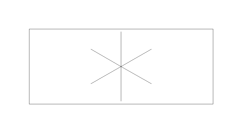
Now onto the recursive step, where the real excitement begins. Having completed one iteration, we’ll set up a loop running from step 2 to n, with each iteration leveraging information from the preceding one to compute its values. Employing the segments(xstart, ystart, xend, yend) call again for drawing the segments simplifies the process. This entails creating x- and y-coordinate vectors for the new segments to be drawn at each step. The starting points’ coordinates are determined by traversing the specified fractional distance, wherebranch, between the previous starting and ending points. As we progress, we must generate a greater number of new segments than before, branching off in both directions from each prior segment while maintaining the original branch active. Consequently, we anticipate the need to generate three times as many new segments as in the previous step.
Code
snowflake <- function(n, nsides=6, angle=60, wherebranch=0.5) {
  plot(NA, xlim=c(-1,1), ylim=c(-1,1), xlab="", ylab="", xaxt='n', yaxt='n', asp=1)
  xstart <- rep(0,nsides)
  ystart <- rep(0,nsides)
  firstangle <- 360/nsides*pi/180
  angle <- angle*pi/180
  xend <- sin(firstangle*(1:nsides))
  yend <- cos(firstangle*(1:nsides))
  segments(xstart, ystart, xend, yend)

  for(i in 2:n) {                                             ##########
    xstart <- rep(xstart + wherebranch*(xend-xstart),3)       ##########
    ystart <- rep(ystart + wherebranch*(yend-ystart),3)       ##########
  }                                                           ##########
}
With the new xstart and ystart values defined, we proceed to determine the ending coordinates by advancing the right distance in the appropriate direction from the starting points. This distance equals the distance from the branching location to the previous endpoint, effectively wherebranch multiplied by itself, as many times as the loop has iterated. Directional calculations involve the angles formed by the previous segments, augmented by the branching angle. As the starting coordinate vectors are replicated three times, we generate coordinate vectors computed by subtracting the branching angle from the previous angles, followed by the previous angles themselves, and finally, the previous angles plus the branching angle. Although the branching angle is user-specified, storing the angles for this iteration’s use in the subsequent iteration is crucial. Additionally, a vector of angles utilized in the initial step must be included.
Code
snowflake <- function(n, nsides=6, angle=60, wherebranch=0.5) {
  plot(NA, xlim=c(-1,1), ylim=c(-1,1),
           xlab="",
           ylab="",
           xaxt='n',
           yaxt='n', asp=1)
  xstart <- rep(0,nsides)
  ystart <- rep(0,nsides)
  firstangle <- 360/nsides*pi/180
  angle <- angle*pi/180
  xend <- sin(firstangle*(1:nsides))
  yend <- cos(firstangle*(1:nsides))

  last_ang <- firstangle*(1:nsides)                                                     ########

  segments(xstart, ystart, xend, yend)
  for(i in 2:n) {
    end_l <- (1-wherebranch)^(i-1)                                                      ########

    xstart <- rep(xstart + wherebranch*(xend-xstart),3)
    ystart <- rep(ystart + wherebranch*(yend-ystart),3)

    xend <- xstart + end_l*c(sin(last_ang-angle),
                             sin(last_ang), sin(last_ang+angle))   ########
    yend <- ystart + end_l*c(cos(last_ang-angle),
                             cos(last_ang), cos(last_ang+angle))   ########

    last_ang <- c(last_ang-angle, last_ang, last_ang+angle)                             ########

    segments(xstart, ystart, xend, yend)                                                ########
  }
}
snowflake(9, wherebranch=.55)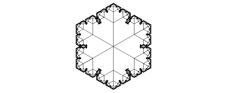
Here it is again with some additional pieces, an logical color argument that prints lines on a rainbow color ramp, and a ... so you can pass in additional plotting arguments. Feel free to add some festive holiday cheer to your office.
Code
snowflake <- function(n, nsides=6, angle=60, wherebranch=0.5, color=T, ...) {
  plot(NA, xlim=c(-1,1), ylim=c(-1,1),
           xlab="", ylab="", xaxt='n',
           yaxt='n', asp=1, ...=...)
  xstart <- rep(0,nsides)
  ystart <- rep(0,nsides)
  firstangle <- 360/nsides*pi/180
  angle <- angle*pi/180
  xend <- sin(firstangle*(1:nsides))
  yend <- cos(firstangle*(1:nsides))
  last_ang <- firstangle*(1:nsides)
  if(color) cols <- rainbow(n)
  else cols <- rep(1,n)
  segments(xstart, ystart, xend, yend, col=cols[1])
  for(i in 2:n) {
    end_l <- (1-wherebranch)^(i-1)
    xstart <- rep(xstart + wherebranch*(xend-xstart),3)
    ystart <- rep(ystart + wherebranch*(yend-ystart),3)
    xend <- xstart + end_l*c(sin(last_ang-angle), sin(last_ang), sin(last_ang+angle))
    yend <- ystart + end_l*c(cos(last_ang-angle), cos(last_ang), cos(last_ang+angle))
    last_ang <- c(last_ang-angle, last_ang, last_ang+angle)
    segments(xstart, ystart, xend, yend, col=cols[i])
  }
}

snowflake(9, angle=70, wherebranch=.45)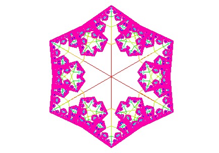
References
‘Fractal Snowflake Models’ by Michael F. Barnsley and John E. Hutchinson.
‘The Formation of Snow Crystals’ by Kenneth G. Libbrecht.
‘Fractal Geometry of Snowflake’ Edges by D. L. Stauffer and A. Aharony.