Beauty in the Midst of Chaos
Random World
Mathematics
Physics
A flap of a butterfly’s wings in Brazil set off a Tornado in Texas
Towards the Chaotic Phenomenon
In August 2017, people across North America planned for an once-in-a-lifetime opportunity to watch a total solar eclipse. Here’s a reference to the 2017 eclipse in an article about a previous one, 99 years earlier.

For centuries, humans have used math and science to make predictions about our universe. Certainly, by the end of the 19th century, scientists felt that we were living in a Cartesian universe, in which, if you had some omniscient being who knew the positions and velocities of all the particles in the universe, in principle, that being would know what would happen for all time.

But if that’s true, why are some things in our world still so hard to predict, even in an era of supercomputers and big data? If we can predict an eclipse a century in advance, why can we only predict the weather about a week or two in advance?
Where Does the Chaos Originate?
Everything Could be Predictable
In the late 1600s, after Issac Newton had come up with his laws of motion and universal gravitation, everything seemed predictable. We could explain the motions of all the planets and moons, and we could predict an eclipse and the appearance of comets with pinpoint accuracy centuries in advance.
The Past Would be Present Before Its Eyes
French scholar and polymath Pierre-Simon Laplace summed it up in a famous thought experiment; He imagined a super-intelligent being, now called Laplace’s demon, that knew everything about the current state of the universe: the positions and momenta of all the particles and how they interact.
“If this intellect were vast enough to submit the data to analysis then the future, just like the past would be present before its eyes”
This is total determinism: the view that the future is already fixed, we just have to wait for it to manifest itself. If you have studied a bit of physics, this is the natural viewpoint to come away with. The Heisenberg principle from quantum mechanics, that’s on the scale of atoms; pretty insignificant on the scale of people. Virtually all these problems could be solved analytically, like the motion of planets, falling objects, or pendulums.
In the case of pendulums, one should understand a fact of a simple pendulum which is phase space. It is one of the most important representations of the dynamical system.
Key Concept of Dynamical System
Dynamical systems involve one or more variables that change over time according to autonomous differential equations.
\(\frac{dx}{dt}=\dot{x}=\) rate of change of \(x\) as time changes
\(\frac{dy}{dt}=\dot{y}=\) rate of change of \(y\) as time changes
\(x\) and \(y\) depend on the independent variable \(t\), which stands for time and the dot notation is special in that it can only be used when the independent variable is time.
For example, \(\dot x = -y-0.1x\) and \(\dot y =y-0.4y\) do not involve \(t\) . It only contains \(x\) and \(y\) as variables. This makes them autonomous; each combination of \(x\) and \(y\) only corresponds to one combination \(\dot x\) and \(\dot y\) .
Some people may be familiar with position-time or velocity-time graphs, but what if we wanted to make a 2d plot that represents every possible state of the pendulum?
Phase Space and Simple Pendulums
Every possible thing it could do in one graph, well on the x-axis we can plot the angle of the pendulum, and y-axis its velocity and this is what is called phase space.
If the pendulum has friction it will eventually slow down and stop and this is shown in phase space by the inward spiral. The pendulum swings slower and less far each time and it does not really matter what the initial conditions are, we know that the final state will be the pendulum at rest hanging straight down, and from the graph, it looks like the system is attracted to the origin, that one fixed point.
Now if the pendulum does not lose energy, well it swings back and forth the same way each time, and in phase space, we get a loop. The pendulum is going the fastest at the bottom but the swing is in opposite directions as it goes back and forth. The close loop tells us the motion is periodic and predictable any time you see an image like this in phase space, you know the system regularly repeats.
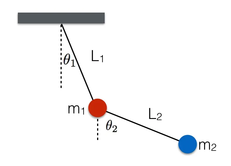
Double Pendulum And Phase Space
We can swing the pendulum with different amplitudes, but the picture in phase space is very similar, just a different-sized loop. Now an important thing to note is that the curves never cross in phase space and that’s because each point uniquely identifies the completion of the system and that state has only one future. So once you’ve defined the initial state, the entire future is determined. This is what is called “Deterministic Chaos”. Deterministic, because its future is determined by physical laws, although it seems random.
Now the mechanics of a pendulum can be well understood using Newtonian physics, but Newton himself was aware of problems that did not submit to his equations so easily, particularly the three-body problem. So calculating the motion of the Earth around the Sun was simple enough with just those two bodies, but add in one more, say the moon, and it became virtually impossible. Newton told his friend Edmond Halley that the theory of the motions of the moon made him a headache, and kept him awake so often that he would think it no more.
Poincare’s Research
In 1903, French mathematician Henri Poincare observed something similar while studying the problem of three objects in space, all affected by each other’s gravity. He was always looking for what’s the most simple set of equations that exhibit chaotic properties. The problem, as would become clear to Henri Poincare two hundred years later, was that there was no simple solution to the three-body problem.
The Motivation of Chaos
Consider the following situations: you are a computer scientist specializing in simulations of dynamical systems such as the weather surrounding your city, or the trajectories of multiple planets affected by each other’s gravitational pulls. This is crucial to your job- you work for the weather forecast, and also part-timer in an intergalactic mastermind’s venture to attack and colonize the Milky Way. Now, as a result of extensive scientific research and your own ingenuity, your simulations can perfectly predict how these systems change over time, given any set of starting parameters. However, you must still be extremely careful in using these simulations to predict what happens in the real world, or else it may result in a widely inaccurate, completely different prediction. This is due to the simple fact that these systems, are chaotic.
Definition of Dynamical System
A dynamical system is a system that has a function that describes the time dependence of a point in a geometrical space. More formally, a dynamical system is defined as a “particle or ensemble of particles whose state varies over time and thus obeys differential equations involving time derivatives”. To predict the system’s future behavior, an analytical solution of such equations or their integration over time through computer simulation is made.
The study of dynamical systems is the focus of dynamical systems theory, which has applications in a wide variety of fields such as mathematics, physics, engineering, biology, chemistry, economics, medicine, and history. They are a fundamental part of chaos theory, logistic map dynamics, bifurcation theory, the self-assembly and self-organization processes, and also the edge of chaos concept.
Pioneer of Chaos
Chaos came into focus in the 1960s, when meteorologist Edward Norton Lorenz tried to make a basic computer simulation of the Earth’s atmosphere. He had 12 equations and 12 variables, things like temperature, pressure, humidity, and so on. And the computer would print out each time step as a row of 12 numbers. So you could watch how they evolved over time.

Now the breakthrough came when Lorenz wanted to redo a run but as a shortcut, he entered the numbers from halfway through a previous printout and then he set the computer to calculate. After a while when he saw the results, Lorenz was stunned.
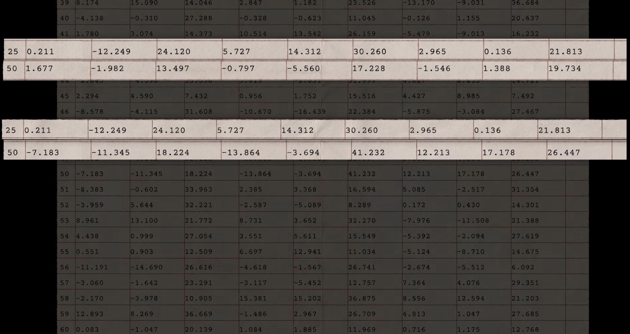
The new run followed the old one for a short while but then it diverged and pretty soon it was describing a different state of the atmosphere (different weather). Lorenz’s first thought, of course, was that the computer had broken (Maybe the Vacuum tube had blown, but none had ). The real reason for the difference came down to the fact the printer rounded to three decimal places whereas the computer calculated with six.
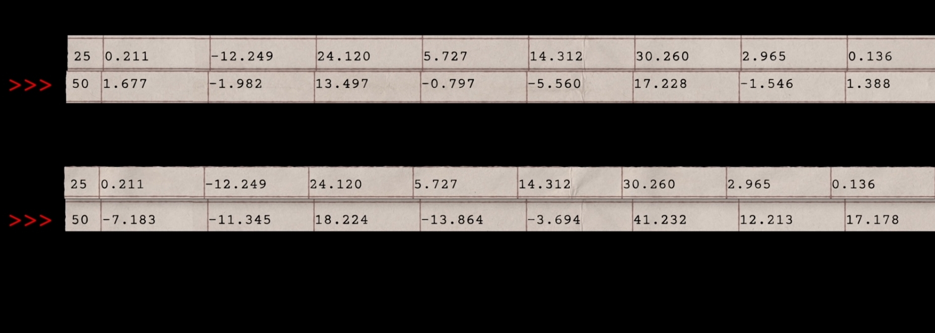
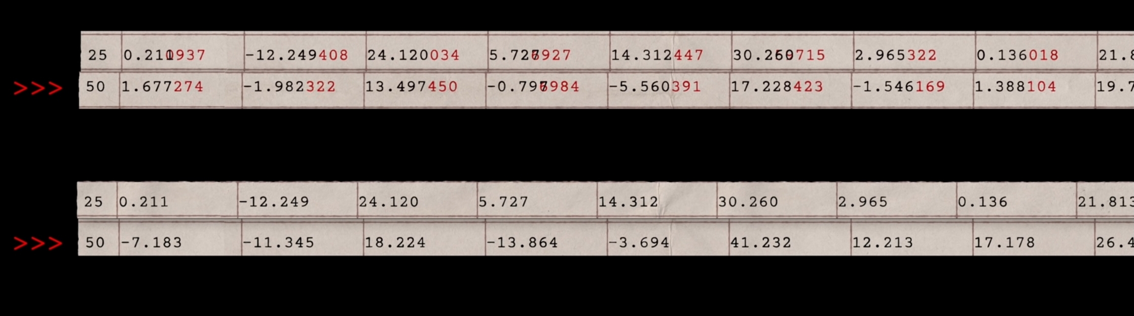
So, when he entered those initial conditions, the difference of less than one part in a thousand created different weather just a short time into the future. Now, Lorenz tried simplifying his equations and then simplifying them some more, down to just three equations and three variables that represent the toy model of convection:
\[\dfrac{dx}{dt}=\sigma(y-x)\]
\[ \dfrac{dy}{dt}=x(\rho-z)-y \]
\[ \dfrac{dz}{dt}=xy-\beta z \]
essentially a 2d slice of the atmosphere heated at the bottom and cooled at the top. But again, he got the same type of behavior; if he changed the numbers just a tiny bit, results diverged dramatically.
Lorenz’s System
Lorenz’s system displayed what’s become known as the sensitive dependencies on initial time conditions, which is the hallmark of chaos. Today we can create models of the atmosphere that go far beyond Lorenz’s columns of numbers.
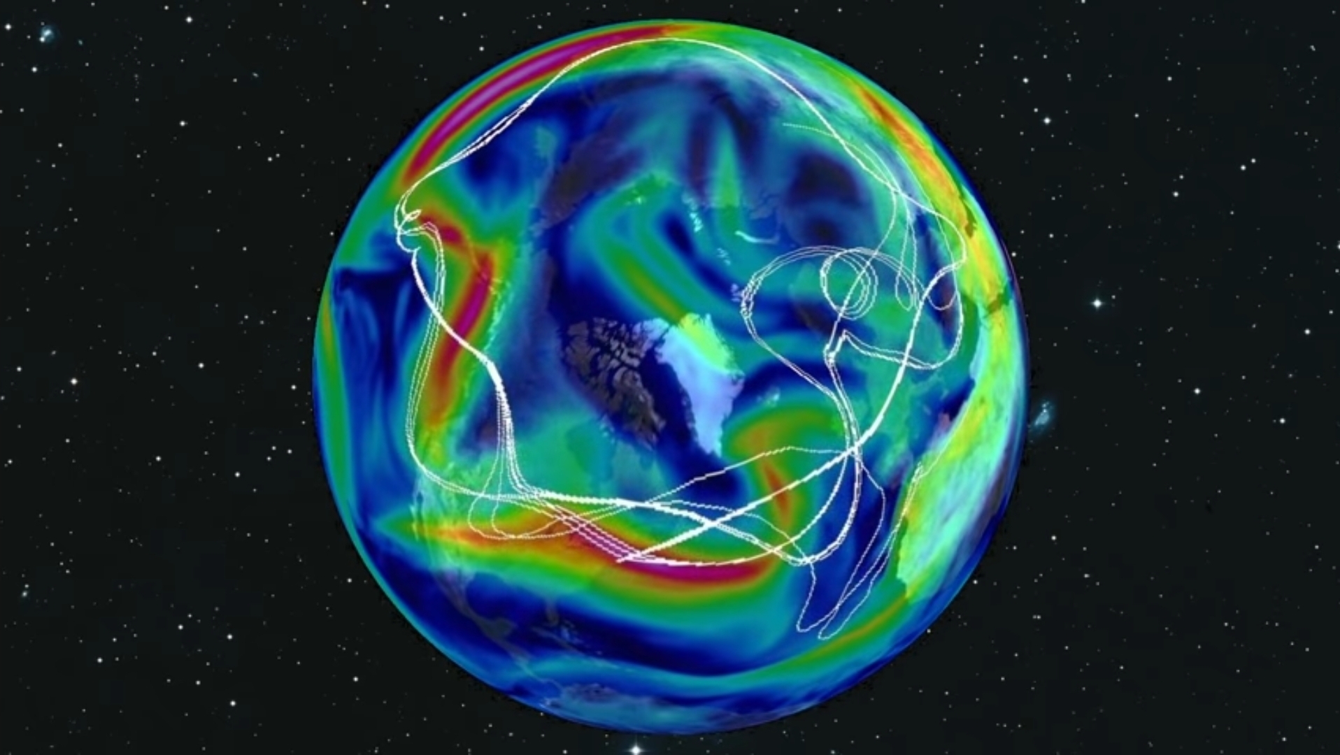
In this model from MIT, the white line represent a bunch of balloons released from approximately the same point. Eventually, the Balloons diverge along very different paths, because of the small differences in their starting points. If you change the initial conditions ever so slightly, infinitesimally slightly. The two trajectories seem to go along with each other and then they diverge exponentially fast. So, that is chaos. It means that you have to know a system with infinite precision to be able to predict it infinitely in time.
Sensitive Dependence on Initial Conditions
When Lorenz found a set of three equations which is the simplified version of equations used to model convection, with only three variables that change over time. It is notable for having chaotic solutions for certain parameter values and initial conditions.\[\dfrac{dx}{dt}=\sigma(y-x)\]
\[\dfrac{dy}{dt}=x(\rho-z)-y \]
\[\dfrac{dz}{dt}=xy-\beta z\]
with the initial conditions : \(x(0)=y(0)=z(0)=1\)
The equations relate the properties of a two-dimensional fluid layer uniformly warmed from below and cooled from above. In particular, the equations describe the rate of change of three quantities with respect to time: \(x\) is proportional to the rate of convection, \(y\) to the horizontal temperature variation, and \(z\) to the vertical temperature variation. The constants \(\sigma\), \(\rho\), and \(\beta\) are system parameters proportional to the Prandtl number, Rayleigh number, and certain physical dimensions of the layer itself where \(\sigma\), \(\rho\), and \(\beta\) are three parameters, with values of \(\sigma = 10,\ \beta= \frac{8}{3}, \rho=28\).
Since Lorenz was working with three variables, we can plot the phase space of his system in three dimensions. We can pick any points as our initial state and watch how it evolves.
It doesn’t seem to. In truth, our system will never revisit the same exact state again. Here I actually started with three close initial states, and they’ve been evolving together so far, but now they’re starting to diverge. From being arbitrarily close together, they end up on totally different trajectories. This is the sensitive dependence on initial conditions in action. Now I should point out that there is nothing random at all about this system of equations. It’s completely deterministic, just like the pendulum. So if you could input exactly the same initial conditions you would get exactly the same result. The problem is, unlike the pendulum, this system is chaotic. So, any differences in the initial conditions, no matter how tiny, will be amplified to a totally different final state. It seems like a paradox, but this system is both deterministic and unpredictable. Because in practice, you could never know the initial conditions with perfect accuracy, and I’m talking infinite decimal places. But the results suggest why even today with huge supercomputers, it’s so hard to forecast the weather more than a week in advance, In fact, studies had shown that by the 8th day of a long-range forecast, the predictions are less accurate than if you just look the historical average for that day and knowing about chaos, meteorologists no longer make just a single forecast, instead, they make ensemble forecasts, varying initial conditions, and model parameters to create a set of predictions. Now far from being the exception to the rule, chaotic systems have been turning up everywhere.
The double pendulum, just two simple pendulums connected together is chaotic here two double pendulums have been released simultaneously with almost the same initial conditions but no matter how hard you try, you could never release a double pendulum and make it behave the same way twice. Its motion will forever be unpredictable.
You might think chaos always requires a lot of energy or irregular motions, but if you imagine a system of five fidget spinners with repelling magnets in each of their arms is chaotic too. At first glance, the system seems to repeat regularly, but if you watch more closely, you’ll notice some strange motions the spinners suddenly flip the other way.
Even our solar system is not predictable. A study simulating our solar system for 100 million years into the future found its behavior as a whole to be chaotic with a characteristic time of about 4 million years which means within say 10 or 15 million years, some planets or moons may have collided or been flung out the solar system entirely.
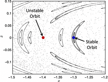
A Brief Introduction to Attractor
Phase Space or State Space
This is a cartesian space where the axes are the system’s variables. Each point in the space is a unique state of the system and has its own rate of change which can be shown as a vector.
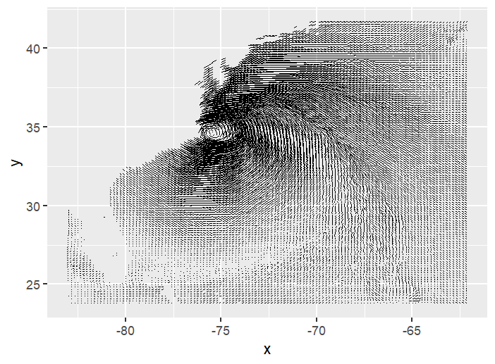
For the specific system shown, the vector field looks like this. Imagine you’re trying to scatter a bunch of random points around to represent different possible states, and you’ll see how they evolve and move around. It seems like they all spiral toward the center.
This brings us to our next topic i.e., attractor
Attractor
An attractor is a set of points in the phase space which attracts all the trajectories in a certain area surrounding it, known as the basin of attraction.
For example, \(\dot x = -y-0.1x\) and \(\dot y =y-0.4y\) , notice that at the origin where \(x=0\) and \(y=0\) , \(\dot x\) and \(\dot y\) is \(0\) too.
Quadratic maps in 2D
We already found some very interesting types of chaotic behaviors. But things get a whole lot more interesting when we consider more than one variable. So let’s move from a single equation to a two-dimensional system of equations with two variables \(x\) and \(y\). In particular, we will focus on what are called two-dimensional quadratic maps, which in their most general form look like this:
\[x_{t+1} = \alpha_1+\alpha_2x_t\ + \alpha_3x_t^2\ + \alpha_4x_ty_t \ + \alpha_5y_t+\alpha_6 y_t^2 \ \ \ \ \ \ \ \ \ \ …(1)\]
\[y_{t+1}= \alpha_{7}+ \alpha_8x_t \ + \alpha_9x_t^2+\alpha_{10}x_{t}y_{t} \ + \alpha_{11}y_t+\alpha_{12}y^2_t \ \ \ \ \ \ …(2)\]
The two variables \(x\) and \(y\) depend on their previous period values in levels and squares as well as the combination of the previous period \(x\) and \(y\). Let’s write a function that takes a starting point \((x_0,y_0)\) and traces its position through each of \(n\) many iterations. Moreover, we will also write a function to plot these points. In this function, we will include an option to drop the first couple of points for which the attractor might not have yet reached its basin of attraction, which is the region where once reached, all future points will wander around in.
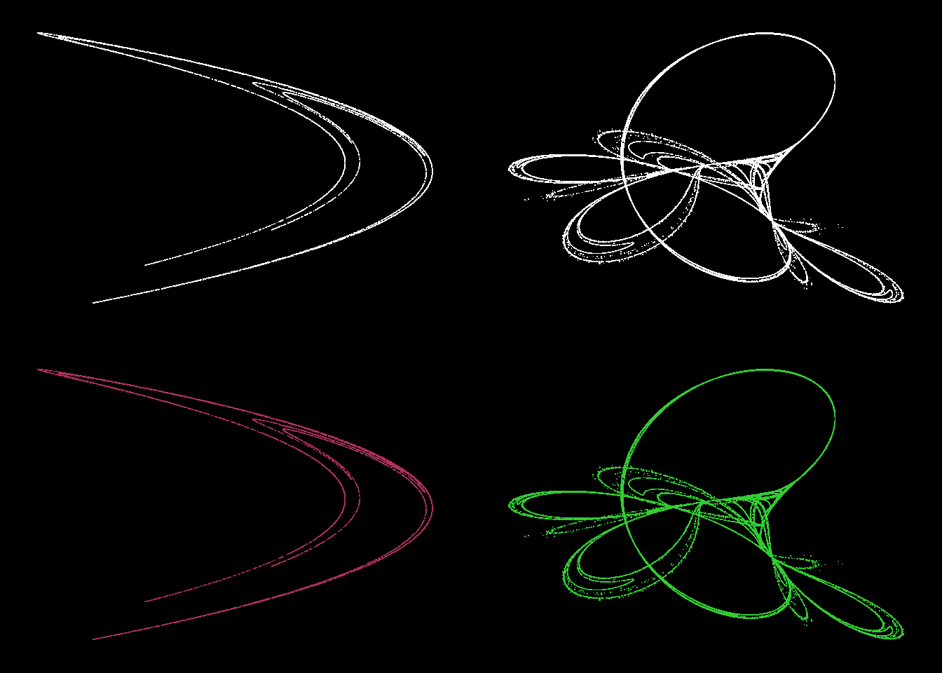
Two Famous Attractor
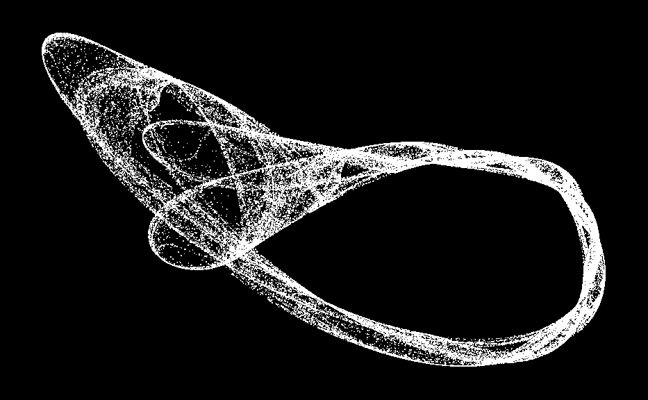
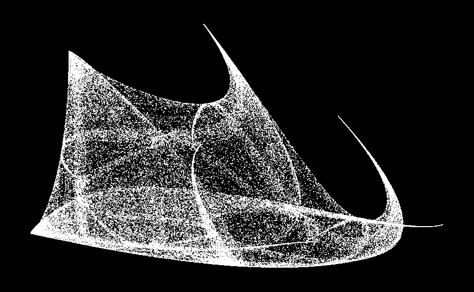
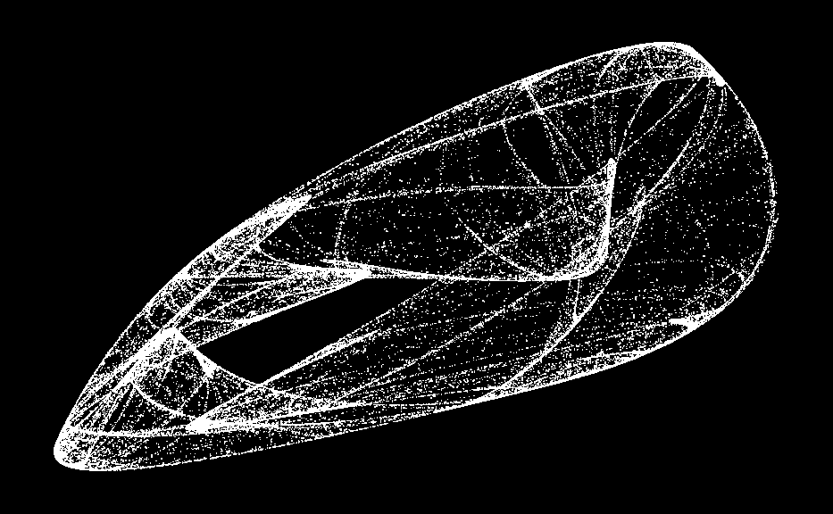
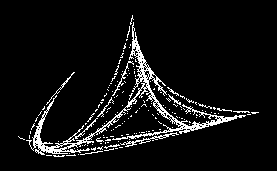
One of the most prominent strange attractors based on a quadratic map is the so-called Hénon map named after French mathematician Michel Hénon. The Hénon map is typically written as
\[x_{t+1}=1-ax^2_t+y_t\]
\[y_{t+1}=bx_t\]
with \(a=0.9\) and \(b=0.3\). Another well-known chaotic quadratic map is the Tinkerbell map, which is commonly written as,\[x_{t+1} = ax_t+by_t+x^2_t-y^2_t\]
\[ y_{t+1} = cx_t+dy_t+2x_ty_t \]
with \(a=0.9, b=−0.6013, c=2\ and\ d=0.5\). Now, all we need to do is to substitute these coefficients into equations (1),(2) and we are ready to plot the first of many hypnotic images. As we programmed different coloring options into our plot function, we can even produce plots with different colors.
Now, a general question will occur that how to relate this things with chaos? So, it is requested to visit here.
Our Own Strange Attractor

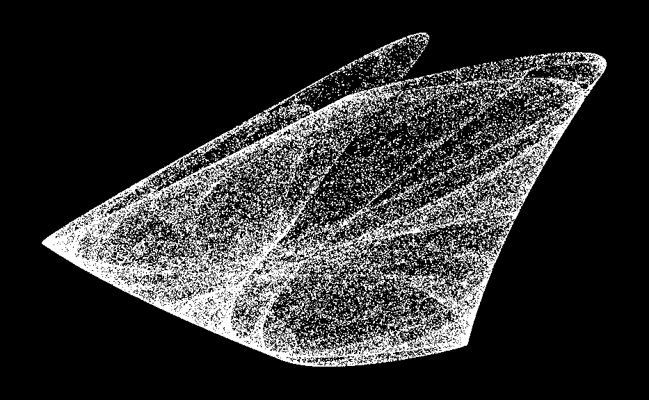
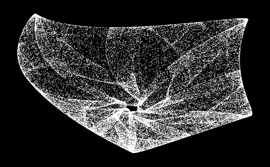

Lorenz Attractor
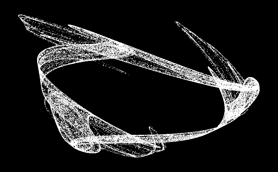
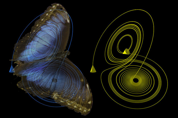
If we specify lorenz equation and plot in three dimensions on a modern computer. The location of the first point is arbitrary. With each point after that, the computer steps forward in time by calculating the position of the next point based on the position of the previous one. It seems to change direction at random, and it never arrives at the same point twice. If it did, that would be the beginning of a repeating pattern. This type of system is now known as a “strange attractor” and this particular one is known as the Lorenz attractor.
It’s the poster child of chaos theory and is sometimes almost synonymous with the butterfly effect or the field of chaos theory itself. It even looks like a butterfly. A strange attractor is one that has a fractal structure. No point in space is ever visited more than once by the same trajectory. If that happened, the trajectory would travel in a predictable loop and no two trajectories will ever intersect. If that happened, they would merge into the same path, giving two different sets of initial conditions the same outcome i.e., a single trajectory will visit an infinite number of points in this limited space, and this limited space will have an infinite number of trajectories.
Trajectories are just curves, so they should be 1-dimensional. But how come no matter how much you zoom in on this attractor, you can always find more and more trajectories everywhere?
This is the reason that this attractor is said to have a non-integer dimension. It’s made up of infinitely long curves in a finite space, which are so detailed that they start to partially fill up a higher dimension. It’s not 1 dimensional, 2 dimensional, or 3 dimensional - it’s dimension is somewhere in between. As a result of this non-integer dimension and detail of arbitrarily small scales, the set of points in the Lorenz attractor is a fractal space, and that’s why it’s a strange attractor.
A strange attractor isn’t necessarily chaotic, but a chaotic attractor will always be strange, and Lorenz attractor is a strange chaotic attractor.
When Lorenz presented his work at a conference in 1963, he ended his talk with an anecdote about a meteorologist who asked whether the flap of a seagull’s wings could change the weather forever. He showed that the appearance of randomness could be well understood within a simple framework of deterministic systems and that it didn’t require excessive complexity at all, it just required one ingredient; the system had to somehow be behaving non-linearly.
Chaos Theory and Butterfly Effect
Butterfly Effect: A Metaphor
This was the major challenge to the idea of the Cartesian Universe. The whole idea that certain systems have these finite prediction horizons that you can’t go beyond which was really new. Nobody imagined that to be the case. When Lorenz presented this work at a conference in 1972, the organizer didn’t receive his talk title in time, so he suggested one:
Does the flap of a butterfly’s wings in Brazil set off a Tornado in Texas?
So, the butterfly instead of a seagull, became the image most associated with his work. It’s had an increasingly profound impact on a number of disciplines. In its first 10 years, Lorenz’s 1963 paper was cited in about 10 other publications. Since then, it’s been cited over 9,000 times, in papers from nearly every field of science.
In 1987, a popular book by James Gleick introduced the world to the work of Lorenz and other Chaos pioneers, and the ‘Butterfly Effect’ became part of popular culture.
The butterfly effect is a theory according to which the smallest thing, such as a butterfly flapping its wings can create a series of events leading to a catastrophe, such as a Tornado. Scientists continue to create mathematical models of more non-linear systems. If those models are correct, deterministic chaos can be found in some fascinating places, including financial markets, as well as the eye movements of people with certain brain disorders; in the onset of sickle-cell disease in the human body; and in the fluctuations of human and animal populations.
How Well Future Can be Predicted
The very system we think of as the model of order is unpredictable on even modest timescales. Now a genuine question occurs in our mind i.e.,
How well can we predict future the future? the answer is, not very well at all at least when it comes to a chaotic system.
The further you try to predict the harder it becomes and past a certain point, predictions are no better than guesses. The same is true when looking into the past of chaotic systems and trying to identify initial causes.

Intuitively, it is like a fog that sets in the further we try to look into the further or into the past. Chaos puts fundamental limits on what we can know about the future of systems and what we can say about their past. But there is a silver lining.
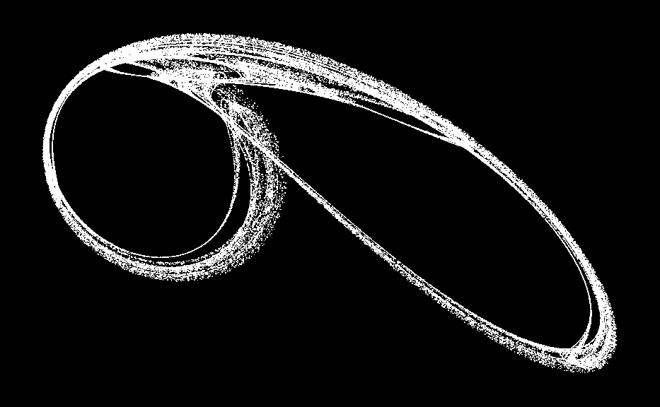
Infinite curve in a finite space
Looking again at the phase space of Lorenz’s equations. If we start with a whole bunch of different initial conditions and watch them evolve, initially the motion is messy. But soon all the points have moved towards or onto an object. The object coincidentally looks a bit like a butterfly. It is the attractor. For a large range of initial conditions, the system evolves into a state on this attractor.
All the paths traced out here never cross and they never connect to from loop, If they did then they would continue on that loop forever and the behavior would be periodic and predictable. So each path here is actually an infinite curve in a finite space.
Lorenz attractor is the most famous example of a chaotic attractor. Though many others have been found for other systems of equations.
Beautiful Structure Underlying Dynamics
If people have heard anything about the butterfly effect, it’s usually about how tiny causes make the future unpredictable, but the science behind the butterfly effect also reveals a deep and beautiful structure underlying the dynamics. One that can provide useful insight into the behavior of a system. So you can’t predict how any individual state will evolve, but you can say how a collection of states evolves and, at least in the case of Lorenz’s equations, they take the shape of a butterfly.
See Also
Footnotes
References
“chaos theory | Definition & Facts”. Encyclopedia Britannica. Retrieved 2019-11-24.
Keydana (2020, June 24). Posit AI Blog: Deep attractors: Where deep learning meets chaos.
Chaos: Making a New Science by James Gleick.
Gilpin, William. 2020. “Deep Reconstruction of Strange Attractors from Time Series.”
Strang, Gilbert. 2019. Linear Algebra and Learning from Data. Wellesley Cambridge Press.
Strogatz, Steven. 2015. Nonlinear Dynamics and Chaos: With Applications to Physics, Biology, Chemistry, and Engineering. Westview Press.
Strogatz, Steven H. (1994). Nonlinear Dynamics and Chaos. Addison-Wesley. p. 262. ISBN 0-201-54344-3.
Luo, Dingjun (1997). Bifurcation Theory and Methods of Dynamical Systems. World Scientific. p. 26. ISBN 981-02-2094-4.
Afrajmovich, V. S.; Arnold, V. I.; et al. (1994). Bifurcation Theory and Catastrophe Theory. ISBN 978-3-540-65379-0.